High performance grid for the metric-calibration of thermographic cameras III / Red de alto rendimiento para la metro-calibration de cámaras termográficas III

Artículo patrocinado por Extraco, Misturas, Lógica, Enmacosa e Ingeniería InSitu, dentro del proyecto SITEGI, cofinanciado por el CDTI. (2012). 

Article sponsored by Extraco, Misturas, Lógica, Enmacosa and Ingeniería Insitu inside the SITEGI project, cofinanced by the CDTI. (2012)

Continúa de: http://carreteras-laser-escaner.blogspot.com/2014/07/high-performance-grid-for-metric.html
Continued from:  http://carreteras-laser-escaner.blogspot.com/2014/07/high-performance-grid-for-metric.html

2.3. Verificación y calibración de parámetros / Verification of calibration parameters

Con el fin de verificar los resultados obtenidos en ambas calibraciones y compararlos con los valores conocidos y certificados, la cámara termográfica calibrada se utiliza para modelar 3D fotogramétrico de un artefacto estándar, con dimensiones conocidas y certificados (Figura 5).

With the purpose of verifying the results obtained in both 

calibrations and comparing them with the known and certified values, the calibrated thermographic camera is used for the photogrammetric 3D modelling of a standard artefact, with known and certified dimensions (figure 5).

Figure 7. Standard artefact consisting of an aluminium block with seven cubes, on top of which five delrin spheres are fixed. Silver and black targets were painted as control points for the photogrammetric restitution, and helping lines were painted with the aim of facilitating image orientation.

El artefacto estándar está formado por un bloque de aluminio con siete cubos de aluminio de dimensiones, en la parte superior que cinco esferas de delrin se pegan con pegamento epoxi, con un diámetro nominal de 100 mm de disminuir. Este artefacto estándar fue calibrado con trazabilidad a la referencia nacional de longitud por una Mitutoyo Euroc Apex 12010 bajo condiciones ambientales controladas en Aimen centro tecnológico (Pontevedra, España) de la máquina de medición por coordenadas. Este dispositivo se utiliza para medir las características geométricas físicas de objetos. Las mediciones se definen por una sonda conectada al tercer eje de movimiento de esta máquina, ya que se compone de tres ejes, x, y y z, ortogonal entre sí en un sistema de coordenadas tridimensional típico. La máquina Lee la entrada de la sonda conmovedora, dirigida ya sea manualmente o por un programa informático y utiliza la x, y coordenadas z de cada uno de estos puntos para determinar el tamaño y la posición. Los resultados obtenidos en esta medida sobre las esferas se muestran en la tabla 3 para facilitar la restitución de punto de los termógrafos adquirido, redondas objetivos fueron pintados en el artefacto estándar. Diferencia de emisividad tomando como base, negros objetivos fueron pintados en el bloque de aluminio, ya que la emisividad de esta pintura es mayor que la del aluminio. Objetivos de la pintura de plata fueron colocados en las esferas de delrin para el mismo efecto, como delrin presenta un mayor valor de emisividad que plata. Dado que las esferas son difíciles de procesar porque su geometría es muy regular, se agregaron algunas líneas para ayudar en la orientación de las imágenes y hacer objetivo identificación más fácil (Figura 7).

Como en el procedimiento de calibración, hay termográficas requisitos que han de tenerse en cuenta. Aunque las diferencias de emisividad son más visibles en las temperaturas altas [26], el artefacto estándar se mantuvo bajo condiciones ambientales de 21 ◦C y humedad relativa de 40%, con las ventanas cerradas y las cortinas para evitar un calentamiento artificial. Dado el valor de baja emisividad del aluminio formando el artefacto, el valor que se utiliza es 0.1, que es el mínimo permitido por la cámara termográfca utilizada en esta prueba. Los modelado 3D termográficos del artefacto estándar se realizó siguiendo los principios de la fotogrametría [15]. Por lo tanto, en la fase de adquisición de la imagen, el artefacto fue dividido en seis modelos: arriba, adelante, abajo; y, como campo de visión de la cámara termográfica no permite la captura de toda la longitud del artefacto en un termógrafo debía dividirse en dos, right–left, con 50% mínimo solapamiento entre modelos consecutivos [27]. Cada modelo consistió en cuatro termógrafos, dos perpendicular al artefacto desde el punto de vista correspondiente y dos con ángulos de 30◦ y 120◦, que podría realizar correctamente ajuste del haz. Termógrafos correspondiente a un modelo se muestran en las figuras 8(a)–(d).Una vez que se adquieren los termógrafos del artefacto estándar, se procesan en software Photomodeler dos veces: una vez con los parámetros de calibración de cámara obtenidos con la rejilla de la base de emisividad de la calibración y luego con los parámetros de calibración con la cuadrícula de calibración de la bombilla. Estos modelos 3D termográficos del artefacto estándar calibrado entonces fueron comparados para evaluar la exactitud y la repetibilidad de las rejillas de calibración diferente, junto con la comparación de resultados de la calibración.

The standard artefact is formed by an aluminium block  with seven aluminium cubes of decreasing dimensions, on top of which five delrin spheres are stuck with epoxy glue, with a nominal diameter of 100 mm. This standard artefact was calibrated with traceability to the national reference of length by a coordinate measuring machine Mitutoyo Euroc Apex 12010 under controlled environmental conditions in Aimen Technological Centre (Pontevedra, Spain). This device is used for measuring the physical geometrical characteristics of objects. Measurements are defined by a probe attached to the third moving axis of this machine, since it is composed of three axes, x, y and z, orthogonal to each other in a typical three-dimensional coordinate system. The machine reads the input from the touching probe, directed either manually or by a computer program, and uses the x, y, z coordinates of each of these points to determine size and position. The results obtained in this measurement concerning the spheres are shown in table 3.

In order to facilitate point restitution from the thermographs acquired, round targets were painted on the standard artefact. Taking emissivity difference as a basis, black targets were painted on the aluminium block, since the emissivity of this paint is higher than that of the aluminium. Silver paint targets were placed on the delrin spheres to the same effect, as delrin presents a higher emissivity value than silver. Given that spheres are difficult to process because their geometry is very regular, some lines were added to help in the orientation of the images and make target identification easier (figure 7).

As in the calibration procedure, there are thermographic requisites that have to be taken into account. Although emissivity differences are more visible at high temperatures [26], the standard artefact was kept under environmental conditions of 21 ◦C and 40% relative humidity, with closed windows and drapes to avoid any artificial heating. Given the low emissivity value of the aluminium forming the artefact, the value used is 0.1, which is the minimum allowed by the thermographic camera used in this test. 

The thermographic 3D modelling of the standard artefact was performed following the principles of photogrammetry [15]. Therefore, in the image acquisition step, the artefact was divided into six models: up, front, down; and, as the thermographic camera’s field of view does not allow the capture of the whole length of the artefact in one thermograph it had to be divided into two, right–left, with 50% minimum overlap between consecutive models [27]. Each model consisted of four thermographs, two perpendicular to the artefact from the corresponding point of view and two with angles of 30◦ and 120◦, so that beam adjustment could be correctly carried out. Thermographs corresponding to one model are shown in figures 8(a)–(d).

Once thermographs of the standard artefact are acquired, they are processed in Photomodeler software twice: once with the camera calibration parameters obtained with the emissivity-based calibration grid, and then with the calibration parameters achieved with the light bulb calibration grid. These thermographic 3D models of the calibrated standard artefact were then compared to evaluate the accuracy and repeatability of the different calibration grids, together with the calibration result comparison.

3. Resultados / Results and discussion

Después de la calibración de la cámara termográfica y la verificación con el artefacto estándar, los resultados se analizaron para evaluar la calidad metrológica del campo calibración propuesto. El análisis se desarrolla por los resultados de calibración métrica y modelado de artefacto estándar

After the thermographic camera calibration and the verification with the standard artefact, the results were analysed in order to evaluate the metrological quality of the calibration field proposed. The analysis is developed for the results of both metric calibration and standard artefact modelling.

Figure 8. Photogrammetric model of the standard artefact: left half, front point of view. Thermographs were acquired orthogonally (a), (b), at 120◦ (c) and at 30◦ (d). Thermographs represent temperatures between 35 and 25 ◦C, as shown in the scale.

3.1. Calibración de parámetros

Los parámetros de calibración obtenidos para la cámara termográfica NEC TH9260 se muestran en la tabla 2. Como puede verse en los valores de desviación estándar, la red basada en la emisividad calibración logra mejores resultados para todos los parámetros que la rejilla de la calibración con bombillas.Distorsión de la lente se obtiene mediante el modelo descentrado (ecuaciones (2), (3)) de distorsión de la lente y desequilibrado radial (ecuación (1)). Estas ecuaciones permiten la corrección de las distorsiones introducidas en las imágenes por la lente de la cámara durante el registro de la imagen

:dr = K1r2 + K2r4 + K3r6, (1)

dpx = P1(r2 + 2x2) + 2P2xy, (2)

dpy = P2(r2 + 2y2) + 2P1xy, (3) 

donde es el radio de la lente, dr la distorsión radial de la lente, dpx decentering distorsión de la lente en el eje x, dpy la distorsión decentering a lo largo del y eje, K1, K2 y K3 son la coefficientsof de la parte radial de la lente distorsión, P1 y P2 los coeficientes de la distorsión de la lente decentering y x e y las distancias de la lente. Teniendo en cuenta los valores obtenidos con ambas calibraciones para los coeficientes K1, K2, K3, P1 y P2, lentes de distorsión resultados fueron comparados para el radio más largo de la imagen. Teniendo en cuenta las coordenadas del punto principal para cada calibración, el radio más largo corresponde a la línea entre el punto principal y la esquina de abajo a la derecha de la imagen (basadas en la emisividad de la calibración) y a la línea entre el punto principal y la esquina superior izquierda (calibración de la bombilla). Los resultados se muestran en las figuras 9 y 10, donde están representadas las distorsiones radiales y decentering como una función del radio. En la misma forma que las cámaras fotogramétricas, radial y descentrar distorsiones aumentan con la distancia al punto principal de la lente.Con el fin de evaluar la consistencia en el cálculo de estos valores de distorsión, el error en el coeficiente de distorsión también se calcula para cada tipo de distorsión de la lente (radial y decentering) y para cada cuadrícula de calibración, con las siguientes ecuaciones para el cálculo de error (ecuación (4) por error en distorsión radial y ecuaciones (5) y (6) por error en descentrar distorsión en x e y ejes):

The calibration parameters obtained for the thermographic camera NEC TH9260 are shown in table 2. As can be seen from the standard deviation values, the emissivity-based calibration grid achieves better results for all parameters than the calibration grid with light bulbs.

Lens distortion is obtained using the unbalanced radial (equation (1)) and decentering (equations (2), (3)) model of lens distortion. These equations allow the correction of the distortions introduced in the images by the camera lens during image registration:

dr = K1r2 + K2r4 + K3r6, (1)

dpx = P1(r2 + 2x2) + 2P2xy, (2)

dpy = P2(r2 + 2y2) + 2P1xy, (3)

where r is the lens radius, dr the radial lens distortion, dpx the decentering lens distortion along the x axis, dpy the decentering distortion along the y axis, K1, K2 and K3 are the coefficients of the radial lens distortion, P1 and P2 the coefficients of the decentering lens distortion, and x and y the lens distances.

Taking into account the values obtained with both calibrations for the coefficients K1, K2, K3, P1 and P2, lens distortion results were compared for the longest radius of the image. Considering the principal point coordinates for each calibration, the longest radius corresponds to the line between the principal point and the down-right corner of the image (emissivity-based calibration), and to the line between the principal point and the upper-left corner (light bulb calibration). The results are shown in figures 9 and 10, where radial and decentering distortions are represented as a function of the radius. In the same way as for the photogrammetric cameras, both radial and decentering distortions increase with the distance to the principal point of the lens.

In order to evaluate the consistency in the calculation of these distortion values, the error in the distortion coefficient is also calculated for each kind of lens distortion (radial and decentering) and for each calibration grid, with the following equations for error calculation (equation (4) for error in radial distortion and equations (5) and (6) for error in decentering distortion in the x and y axes):

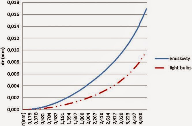Figure 9. Radial distortion obtained from the evaluation of the radial distortion equation with the coefficients obtained with both calibration grids, the proposed one (based on emissivity differences) and the most common one (made with light bulbs).

donde udr es el error de distorsión radial, udpx y udpy son los errores en descentrar distorsión en x y y ejes, uKi es la desviación estándar en el cálculo de coeficientes Ki en cámara calibración y uPi es la desviación estándar en el cálculo de coeficientes de Pi. Teniendo en cuenta las ecuaciones de distorsión (ecuaciones (1)–(3)), las ecuaciones de error final utilizadas fueron los siguientes:

where udr is the error in radial distortion, udpx and udpy are  the errors in decentering distortion in the x and y axes, uKi is  the standard deviation in the calculation of Ki coefficients  in camera calibration and uPi is the standard deviation in the calculation of Pi coefficients. Considering the distortion equations (equations (1)–(3)), the final error equations used were the following:

Los resultados de estos errores en función del radio más largo en cada calibración se graficaron en las figuras 11 y 12. Como ocurre con los otros parámetros de calibración, los valores obtenidos a través de la calibración automática con la rejilla de la base de emisividad calibración son más precisos que los obtenidos con la red de calibración de bombilla, ya que el error en la distancia máxima para la primera red hasta el punto principal es un tercio de la de la segunda distorsión radial y descentrar la distorsión en el eje xy un cuarto para descentrar la distorsión en el eje y.

The results of these errors as a function of the longest radius in each calibration are graphed in figures 11 and 12. As happens with the other calibration parameters, the values obtained through the automatic calibration with the emissivity-based calibration grid are more accurate than those obtained with the light bulb calibration grid, since the error in the maximum distance for the first grid to the principal point is one third of that of the second for radial distortion and decentering distortion in the x axis, and one quarter for decentering distortion in the y axis.

Figure 10. Decentering lens distortion obtained from the evaluation of the decentering coefficients in both axes x (a) and y (b), resulting from the calibration with the emissivity and the light bulb calibration grids.

Figure 11. Error obtained in the calculation of the radial distortion parameters with both calibration grids.

Continúa en: http://carreteras-laser-escaner.blogspot.com/2014/07/high-performance-grid-for-metric_9.html

Continued on: http://carreteras-laser-escaner.blogspot.com/2014/07/high-performance-grid-for-metric_9.html

For more information or if you prefer this article in pdf-format, contact with us:

http://carreteras-laser-escaner.blogspot.com.es/p/contacte-con-nosotros.html

Or, send us an e-mail.