Coordinates in fractals systems / Coordenadas en sistemas fractales

Previo: Situando un punto relativo en una recta:/ Previous: Placing a relative point on a line:

Nos parece muy claro cómo definir un punto situado en una recta. El sistema es sencillo. Se elige un punto al que se denominará origen Y una dirección como positiva. En este entorno se le hace corresponder un punto con la distancia al origen. A ésta distancia se le dará un signo dependiendo del sentido con la dirección prefijada. Es obvio:

It seems very clear how to define a point on a line. The system is simple. A point is chosen. It is called the origin and a direction as positive. In this environment is made to correspond a point with distance from the origin. At this distance will be given a sign depending on the direction to the given address. It is obvious:

Basta con decir: 2.156 y ya hemos situado el punto en la recta:
It is suficente to say: 2.156 and have already placed the point on the line:

Previo: Situando un punto relativo en un plano: / Previous: Placing a relative point on a plane:

De igual manera, colocamos un punto como origen dos direcciones no coincidente y la pareja distancias que sigan estas direcciones será la definición del punto:

Similarly, as we place a point source, and two different directions. The two distances to follow these directions will define the point:

El punto sería el P (2.156, 3.987) con ese origen y ejes.
The point would be P (2.156, 3.987) with the origin and axes.

Definición de la posición relativa de un punto en un fractal: / Definition of the relative position of a point in a fractal:

A priori, esto no parece tan sencillo:
A priori, it does not seem so simple:

¿Cómo especificamos un punto es esta forma? Si la dimensión de este fractal estará entre 1 (son líneas) y 2 (se desarrolla en un plano)  ¿Cómo sitúo un punto con sólo 1 ó 2 números reales?

How to specify a point is this way? If the dimension of this fractal be between 1 (are lines) and 2 (developed in a plane). How do I place a point with only 1 or 2 real numbers?

¿Puedo definir un punto como origen? Esta parte es fácil. Basta con coger cualquiera.

¿Qué debe(n) significar el(los) número(s) que le acompañen?

Can I define a point as the origin? This part is easy. Just take any.
What should mean number(s) that will accompany it?

1ª Abstracción: Conversión de un número real una sucesión de números enteros. / 1st Abstraction: Conversion of a real number a sequence of integers.

Siguiendo el primer ejemplo, el Punto P se define como el situado a 2.156860214... unidades del origen. También se podría decir que el número es el definido por la sucesión entera {2, 5, 6, 8, 6, 0, 2, 1, 4, ...} en clave decimal. (para 20.345... correspondería la sucesión: {20, 3, 4, 5, ...})

Para 2D la sucesión para P(2.156..., 3.987...) sería ({2, 1, 5, 6,...}, {3, 9, 8, 7,...}) (en clave decimal)

Si partimos de nuestro fractal:

Following the first example, the point P is defined as. the located 2.156860214 ... units from the origin. One could also say that the number is defined by the entire sequence {2, 5, 6, 8, 6, 0, 2, 1, 4, ...} in decimal code. (20,345 ... correspond to the sequence: {20, 3, 4, 5, ...})

For 2D, the sequence of P (2156 ... 3987 ...) would be ({2, 1, 5, 6, ...}, {3, 9, 8, 7, ...}) (in decimal code)

If we start our fractal:

Partiendo del origen, tenemos que retroceder una espiral (-1) , Avanzar 12, entrar y avanzar 1, y en esa línea moveros 0.2753... unidades (por ejemplo).
Las coordenadas PF serán {(-1, 12, 1, 0[ ...]) (0, 2, 7, 5, 3, ...)}

Starting from the origin, we must go back a spiral (-1), Advance 12 to enter and advance 1 and in that vein, we move 0.2753 ... units (for example).
PF will be the coordinates {(-1, 12, 1, 0[...]) (0, 2, 7, 5, 3, ...)}

Nota:  0[ ...] significa: sucesión infinita de ceros.
Note: 0[...] means infinite sequence of zeros.

La diferencia fundamental con un punto definido en un plano es que los valores de P, 2.156... y 3.987..., son igualmente importantes. En cambio, para P(fractal) la primera sucesión (-1, 12, 1) hace que cuanto más larga sea menos importa la precisión del segundo factor real, (0.2753). Es decir, en un plano si se desea tener una precisión (o error máximo de e) podremos poner 1, 2, ... ó 27 decimales si e = 10^-27. Pero en el caso de PFractal nos pueden ocurrir dos cosas:

• Si tenemos un número suficientemente elevado de elementos de la primera sucesión sea por ejemplo:  (2, 8, 5, 6, 7, 3, 5, 4, 68, 54, 2, 10, 9) el valor real puede, hasta llegar a ser incluso innecesario.

• Al contrario, ante un número muy corto en la sucesión primaria (2, 8) haría falta un valor de la parte real muy precisa para llegar a la misma precisión que en el caso anterior.

The fundamental difference with a defined point in a plane is that P values (2.156 ... 3.987 ...) are equally important. However, for P (fractal) the first sequence (-1, 12, 1) makes the longer it is, the less important the precision of the second real factor (0.2753). That is, in a plane if you want to be accurate (or maximum error e) we can put 1, 2, ... or 27 decimal places (if e = 10^-27). But if PFractal two things can happen:

• If we have a sufficiently large number of elements in the first sequence. eg (2, 8, 5, 6, 7, 3, 5, 4, 68, 54, 2, 10, 9), the actual value can, to become even unnecessary.

• Conversely, when a very small number in the primary sequence, eg (2, 8) would take a value of the real part very accurate to reach the same precision as in the previous case.

¿cómo sabemos calcular precisiones idénticas? ¿Qué se extrae de todo esto? / How do we calculate identical accuracies? What is extracted from all this?

Para amenizar el momento os pongo un vídeo:
To entertain I put a video:

Otherwise:

2º  Trabajo, realizar un programa que trabaje para nosotros: / 2nd abor, make a program that works for us:

Para hacer este fractal hemos utilizado VB, con esta subrutina:
To make this fractalwe have used VB with this subroutine:

Sub PINTA(ByVal XI As Double, ByVal YI As Double, _
          ByVal RI As Double, ByVal ANGINI As Double, _
          ByVal FONDO As Integer)
lim = 10

'Si nos salimos de los límites del dibujo
If FONDO > 0 Then If XI < -2000 Or YI < -2000 Or XI > Picture1.ScaleWidth + 2000 Or YI > Picture1.ScaleHeight + 2000 Then Exit Sub

'Definiciaón de la penetración máxima
If FONDO > lim Then Exit Sub


If FONDO > 5 Then QBColor (FONDO - 4) Else colo = QBColor(FONDO + 10)

'Establecimiento de los valores iniciales
A = 0: r = RI: Y = YI: X = XI: X1 = X: Y1 = Y: RESTO = 0: i = 0
Do
  X = X + r * Cos(i + ANGINI): Y = Y + r * Sin(i + ANGINI)
  Picture1.Line (X, Y)-(X1, Y1), colo
  If i >= RESTO Then
    RESTO = RESTO + 0.6
    PINTA X, Y, r / 4, i + ANGINI + 0.05, FONDO + 1 
  End If
  X1 = X: Y1 = Y: i = i + 0.1: r = r * 0.99
Loop Until r < 2
End Sub

En nuestro formulario de VB hemos añadido un objeto Picture (llamado Picture1) para que funcione. 

La orden inicial es PINTA , X0, Y0, R0, 0 ' R0=660, espiral inicial

In our VB form we have added a Picture object to work (called Picture1).
The initial order is PINTA, X0, Y0, R0, 0 ' R0=660,  inicial value)

3º  Precisiones extremas / extreme accuracies

En la solución de las coordenadas prevista:
In the solution of the provided coordinates:

                       {(A₁, A₂, …, A_n), M ± e} con A_i Î  y M Î 
                       Se buscará la relación entre n y e.
                       The relationship between n and e is searched.

Cuando existe una bifurcación, hay dos posibilidades:
When a bifurcation there are two possibilities:

1. Continuar por la espiral en la que estamos, o,
2. Entrar en una nueva espiral por el extremo inicial de ésta.

1. Continue along the spiral in which we are, or,
2. Enter into a new spiral from the starting end of it.

Si continuamos por la espiral por la que hemos empezado, no haremos nada más difícil que recorrer una "recta enrrollada" luego para una e = 10^-5  tendremos la íltima precisión en el decimal 5.

If we continue along the spiral for which we have begun, we will do nothing more difficult to travel a "curve-straight" then for e = 10^-5 have the íltima fifth decimal accuracy.

       -> Precisión 1  = log(e )/log(10)

El otro extremo es rentrar en una espiral, y otra, y otra... y así sucesivamente. Cada vez que se hace eso, el radio se reduce a la cuarta parte, y así sucesivamente cada vez que penetramos en una nueva espiral. En "n" veces seguidas: : e = R₀/4ⁿ . Si despejamos n: n =  Int[ log(R₀) - log(e) ] / log(4). Ya tenemos la relación buscada:

The other possibility is to go into a spiral, and within another, and within another ... and so on. Every time you do that, the radius is reduced to a quarter, and so on every time we enter a new spiral. In "n" times in succession: e = R₀/4ⁿ. Solving for n: n =  Int[ log(R₀) - log(e) ] / log(4). We already have the required relation:

       -> Precisión 2 = Int[ log(R₀) - log(e) ] / log(4)

Tabla con varios valores de  e: (R₀ = 660, valor inicial)
Table with several values of  e: (R₀ = 660, inital value)

     Dado e   → espiral n máxima    , nº decimales máximos

           1 → 4.68316110 » 5      ,        1

         0.1 → 6.34412515 » 7      ,        2

        0.01 → 8.00508920 » 9      ,        3

       0.001 → 9.66605325 » 10 (*) ,        4

      0.0001 → 11.3270173 » 12 (*) ,        5

     0.00001 → 12.9879813 » 13 (*) ,        6

    0.000001 → 14.6489453 » 15 (*) ,        7

   0.0000001 → 16.3099094 » 17 (*) ,        8

                  e → 

   Int(-1,661*log(e)/log(10) + 4,6832),    log(e)/log(10)

Cada vez tiene menos importancia el valor inicial de R₀ frente al valor creciente de log (e).

 (*) Ojo: hay dos dígitos, lo cual hace ver que se necesita uno más.

Gradually becoming a less significance the initial value of R₀ against the rising value of log (e).

  (*) Caution: there are two digits, which makes it look that is needed one more.

     Dado e   → espiral n máxima    , nº decimales máximos

           1 →              5      ,        1

         0.1 →              7      ,    2

        0.01 →              9      ,        3

       0.001 →             11      ,        4

      0.0001 →             13      ,        5

     0.00001 →             14      ,        6

    0.000001 →             16      ,        7

   0.0000001 →             18      ,        8

-1,661*log(e)/log(10) + 4,6832 + log(-1,661*log(e)/log(10) + 4,6832)/log(10)

4º  Comparación con el plano / Comparison with a plane

Si pudiéramos comparar este sistema de coordenadas relativo de forma coherente con el sistema de coordenadas relativo a un plano y/o recta, estaríamos más cerca de poder definir la dimensión fractal.

If we could compare the relative coordinate system in coherence with the coordinate system on a plane and / or a line, we would be closer to define the fractal dimension.

Próximamente su conclusión.
Coming soon its completion.

IRI "low cost"

Creación de un IRI "low cost" (es decir, barato) / Creating an IRI "low cost" (ie cheap)

La idea de crear un aparato que mida el IRI y cueste poco es sencilla si partimos de varias nociones iniciales. The idea of creating a device that measures the IRI and its being cheap is simple if we start from several initial notions.

1º Saber como debe medir un IRI / We need to know how it should measure an IRI

El principio fundamental es el denominado "modelo de cuarto de coche": / The fundamental principle is called "golden-car:

Modelo de cuarto de coche

Para saber más: More information:

• http://es.wikipedia.org/wiki/Índice _de_regularidad_internacional
• http://www.carreteros.org/normativa/otros/nlt/pdfs/rosas/1998/330_98.pdf

2º Saber como se montan las ondas (las que queremos medir y las que queremos eliminar, ruido). Introducción matemática del modelo reductor de vibraciones transmitidas por el vehículo / Knowing how to ride the waves, (which we measure and we want to eliminate noise). Mathematical reduction vibration model vehicle.

Primeramente vamos a establecer las bases de nuestro discurso con una revisión de la transmisión de información asociada a ondas. Hay dos formas de realizar tal transmisión, por modulación de amplitud y por modulación de frecuencia.

En la modulación de amplitud se suman las ondas de diferente frecuencia:

First, we will establish the foundations of our discourse with a review of the transmission of information associated with waves. There are two ways to perform such transmission, amplitude modulation and frequency modulation.

In amplitude modulation, different frequency waves are added:

Dos ondas de diferente frecuencia

Suma de ondas (an amplitud)

La amplitud de la onda portadora (alta frecuencia) se moldea según el patrón de la onda señal (baja frecuencia.

En el caso de la frecuencia modulada se variará la frecuencia según el patrón de la señal:

The amplitude of the carrier wave (high frequency) is molded according to the pattern signal wave (low frequency.

In the case of frequency modulation, the frequency will vary the signal pattern:

Variando la frecuencia de una en función de la otra

Las transmisiones de onda media tiene las siguientes características generales: La propagación en esta banda sigue la curvatura de la Tierra, y las ondas pueden reflejarse en la ionosfera pero es sumamente vulnerable al ruido atmosférico y al producido por maquinaria y aparatos eléctricos.

Edwin Armstrong presentó su estudio: "Un Método de reducción de Molestias en la Radio Mediante un Sistema de Modulación de Frecuencia" (1936). La FM de requiere un mayor ancho de banda que la modulación de amplitud para una señal moduladora equivalente, pero a su vez hace a la señal más resistente al ruido y la interferencia. La modulación de frecuencia es también más resistente al fenómeno del desvanecimiento, muy común en la AM. Por estas razones, la FM fue escogida como el estándar para la transmisión de radio de alta fidelidad.

Medium wave transmissions have the following general characteristics: Propagation in this band follows the curvature of the Earth, and waves can reflect off the ionosphere but is highly vulnerable to atmospheric noise and produced by electrical machinery and apparatus.

Edwin Armstrong presented his study: "A method for reducing discomfort Radio System Using a Frequency Modulation" (1936). The FM requires a wider bandwidth than the amplitude modulation signal for modulating an equivalent, but in turn renders it more resistant to noise and interference signal. Frequency modulation is also more resistant to fading phenomenon, common in the AM. For these reasons, the FM was chosen as the standard for transmitting high fidelity radio.

Diagrama electrónico de un receptor básico de AM

Otra de las grandes diferencias entre la modulación de amplitud y frecuencia es respecto a la complejidad del receptor. No hay nada más simple que un receptor de AM (imagen). La desmodulación es muy simple y, por consiguiente, los receptores son sencillos y baratos , todo esto gracias a Robert Herzenbert que en 1932 patentó el término AM; un ejemplo de esto es la radio de galena.

Con lo que se concluye que la AM es más sencilla, se transmite y entiende mejor pero añade ruido. La FM sólo aporta la ventaja de la inmunidad frente al ruido electromagnético.

Another difference between the amplitude and frequency modulation is receiver complexity. There is nothing simpler than an AM (image). Demodulation is very simple and therefore, the receivers are simpler and cheaper, all this thanks to Robert Herzenbert in 1932 patented the term AM; An example of this is the crystal radio.

Thus we conclude that the AM is simpler, transmitted and understood better but adds noise. The FM only provides the advantage of immunity to electromagnetic noise.

3º Estudio de la transmisión con la señal con amortiguación / Study of the transmission signal with damping

Impacto amortiguado / Damped impact

El típico reflejo del movimiento de la masa sobre muelle y amortiguador es el siguiente. Como se observa el amortiguador actúa sobre la amplitud pero no sobre la frecuencia.

La diferencia radica ante otro escalón. No sólo se rompe la amplitud, también la frecuencia.

The typical reflection of movement of the mass on the spring and damper is the following. As the damper acts on the amplitude but not the frequency is observed.

The difference is before another step. Not only breaks the amplitude, frequency also.

Amortiguación de dos impactos / Double damped impact

El punto importante es que en el caso anterior, 1 escalón produce 1 diferencia de frecuencia y 5 resaltos en amplitud apreciables con la vista (resaltos que no existen el el suelo). Y en el caso contiguo tenemos 2 escalones, 2 cambios de frecuencia y algunas subidas de amplitud (inexistentes).

Si además se añade ruido (vibración del vehículo), Como en la AM añadiremos una señal sinusoidal de baja intensidad relativa:

The important point is that in the former case, one step produces 1 frequency difference and five projections in appreciable extent to view (no protrusions that the soil). And in the next case we have 2 steps, 2 changes of frequency and amplitude uploaded some (nonexistent).

If also noise (vibration of the vehicle) is added, as in the AM add a sinusoidal low signal intensity on:

Tan “sólo” hubo que averiguar que resulta mas sencillo y/o fiel para el filtrado de la vibración portadora (vibración propia del vehículo) y extracción de la señal que nos interesa.

So "only" had to find out which is easier and / or true for filtering the carrier vibration (natural vibration of the vehicle) and obtaining the signal of interest.

4º Modelo matemático de eliminación de errores / Mathematical model debugging

La AM corresponde a la función:

       a = A(x) · seno (w_at+f_a) · sen0(w_dt+f_d);

a: aceleración resultante.

A(x): amplitud en función del espacio

w_a: frecuencia propia del auto

w_d: frecuencia propia de la señal (derivada del amortiguador)

La FM corresponde con la función:

       a = A(x) · seno (w_at + f_a + f(w_dt + f_d));

a: aceleración resultante.

A(x): amplitud en función del espacio

w_a: frecuencia propia del auto

w_d: frecuencia propia de la señal (derivada del amortiguador)

f: función de interferencia.

Los condicionantes externos son esenciales ante el movimiento vibratorio propio del conjunto masa(s) + muelle(s) + amortiguador(es). Éstos son, la definición del terreno, señal de estudio, y la vibración natural del vehículo. La primera debería ser un invariante, dado que es lo que se quiere evaluar y la segunda será dependiente del propio vehículo, la velocidad de éste (aumenta con la velocidad), marcha en la que se encuentre (baja si sube la marcha).

Matemáticamente, si quisiéramos extraer la información a partir de la vibración resultante transmitida según un modelo de amplitud modulada, lo primero sería obtener la variación de la amplitud propia en función de la velocidad del vehículo para eliminarla.

Vamos a tomar un número muy significativo de datos. Aún así va a sernos muy difícil la extracción de las frecuencias propias (w_a) y los desfases (f_a). Por ello, resulta muy importante analizar los datos extraídos, sus análisis estadísticos, y trataremos de analizar la señal en las crestas y jugar de esta manera sólo con las amplitudes. Evitaremos así, la realización de estudios más complejos como Foucault o similares.

The external factors are essential against self vibratory motion of the mass assembly (s) + spring (s) + damper (s). These are: the definition of the terrain, signal study, and the natural vibration of the vehicle. The first should be an invariant, since it is to be evaluated and the second is dependent on the vehicle itself, the speed of this (increases with speed), and gear in which (low if you upload the gear) 

Mathematically, if we extract the information resulting from the vibration transmitted in a pattern of amplitude modulation, the first thing would obtain the variation of the amplitude versus own vehicle speed to remove.

We will take a significant amount of data. Still it very difficult to extract the natural frequencies (w_a) and the offsets (f_a). Therefore it is very important to analyze the extracted data, statistical analyzes, and try to analyze the signal the crests and play this way only the amplitudes. We will avoid performing more complex studies as Foucault or similar.

5º Análisis de la señal desde el punto de vista de la amplitud modulada.

Para el registro del datos partimos de dos vibrómetros pegados al chasis en cada lado de las ruedas traseras. Están conectados a un dispositivo Arduino que se encarga de digitalizar la señal analógica y transmitirla al puerto serie. La velocidad de transmisión es de 115.500 B/s (la más alta posible). Por otro lado contamos con un GPS que además de transmitirnos las coordenadas nos dará el dato de la velocidad del vehículo. Este punto en importante porque ya que podemos contar con el dato del tiempo transcurrido podremos tener una especie de “odómetro vía satélite”.

Cada vez que tenemos un dato nuevo de posición y velocidad guardamos estos y los datos del buffer del puerto serie del dispositivo Arduino. Éstos tiene esta forma:

To register the data we start from two vibration meters glued to the chassis on each side of the rear wheels. They are connected to an Arduino device that is responsible for digitizing the analog signal and transmit it to the serial port. The transmission speed is 115.500 B / s (the highest possible). Furthermore they have a GPS coordinates addition we will transmit the data of the vehicle speed. This important point because we can count the elapsed time data can have a "odometer via satellite".

Whenever we have a new position and velocity data and store these data buffer Arduino serial port device. They have this form:

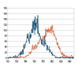
764.00,802.00

759.00,802.00

767.00,800.00

766.00,796.00

768.00,798.00

---

Gráfica de los datos anteriores (rojo:izda., azul:dcha.)

En este caso en particular estaríamos hablando de 900 puntos sólo en 14 metros, 1 dato cada 15 cms, ó, 64 datos/metro.

Para la extracción de nuestra variación de la amplitud, lo primero será saber cuales son las amplitudes máximas que le corresponden dependientes de la velocidad de la frecuencia 'portadora'. Den nuestro caso, después de varios ensayos (después de recorrer cientos de kms a diferentes velocidades por todo tipo de vías).

De los datos se diferenciaran a grupos por velocidades y se elaborarán sus respectivas 'campanas de Gauss'.

In this particular case we are talking about 900 points just 14 meters, 1 data every 15 cm, or 64 data / meter.

For the extraction of our amplitude variation, the first step is to know what the maximum amplitudes that are dependent on the speed of the 'carrier' frequency. Den our case, after several trials (after traveling hundreds of kilometers at different speeds for all types of roads).


Data groups differed by their respective speeds and 'bells Gauss' will be developed.

A 40 km/hora	A 60 km/hora
A 50 km/hora	A 70 km/hora

De estos valores se extrae la media y los valores de umbral al 5%. Es decir, nos responderemos a la pregunta ¿a partir de que valor estamos en una vibración forzada, en una señal?. Después de varios ensayos encontramos una función bastante simple, en función de la velocidad:

si A_i  ã +-± 0,3 · v_i.; ã: amplitud media

The average of these values and the threshold values is extracted 5%. That is, we respond to the question from that value are in a forced vibration in a sign ?. After several tests are quite simple function, depending on the speed:

if A_i  ã +-± 0,3 · v_i.; ã: mean amplitude

v_i.: velocidad en el punto i

A_i: amplitud en el punto i

No sólo el umbral es función de la velocidad. También lo es la propia amplitud. A mayor velocidad mayor es la vibración transmitida y este dato hay que minorizarlo en consonancia. Para ello se realizan varias mediciones en en mismo tramo de carrera a diferentes velocidades y se extrae la relación entre aumento de amplitud y aumento de velocidad:

Escala_velocidad = -0,085 · v_i.+ 9,4

The threshold is not only a function of speed. So is the amplitude itself. The greater the velocity is transmitted vibration and this fact must be minorizarlo accordingly. To do this in multiple measurements are taken in the same stroke length at different speeds and the relationship between amplitude and increase extracted speed increase:
Speed Scale = -0.085 · v_i.+ 9.4

Nuestro parcial en la obtención del IRI sera: / Our partial measure in obtaining the IRI will:

S = Σ | pk_i+1 - pk_i | · (-0,085 · v_i.+ 9,4)

y por tanto: / and therefore:

IRI_100m=Σ | pk_i+1- pk_i | · (-0,085 · v_i.+ 9,4) / Σ | pk_{i +1} - pk_i |

Siempre y cuando. Whether Σ | pk_{i +1} - pk_i | = 100.

Exponemos los resultados de dos ejemplos (Omitimos el nombre de la carretera estudiada):
We present the results of two examples (We omit the name of the road studied):

IRI a la ida (superior) y vuelta (inferior) / IRI on the way (top) and back (bottom)

Respecto a los valores estadísticos. El láser daba: medias de 1,77 y 1,79 y el nuestro 1,86 y 1,90. Las varianzas eran de 0,60 y 0,80.

Regarding the statistical values. The laser was: averages of 1.77 and 1.79 and 1.86 and 1.90 ours. The variances were 0.60 and 0.80.

Otra carretera: / Another road:

6º Entendido como funciona la matemática vamos a crear el prototipo real / Understood as mathematical functions we create the actual prototype

Con todo lo que habíamos avanzado nos propusimos la creación de un sistema de medición del IRI más económico. Estaría basado en un par de vibrómetros, un Arduino, un GPS de bajo coste y un ordenador portátil. El coste fue de 25€ por vibrómetro, 25€ el Arduino y el GPS ya lo teníamos en la empresa y su costo fue de 250€.

Colocación del instrumental:

With all that we had gone we proposed the creation of a measurement system cheaper IRI. It would be based on a pair of vibration meters, an Arduino, low cost GPS and a laptop. The cost was 25 € per vibrometer 25 € the Arduino and GPS already had on the company and its cost was 250 €.



Instrument positioning:

Colocación del instrumental

El vibrómetro se coloca en la zona roja de la figura anterior. Uno al lado de cada rueda.

The vibrometer is placed in the red zone of the previous figure. One side of each wheel.

Sensor "low cost"

Montaje

Arduino antes y después del montaje

Los vibrómetros se conectan al Arduino del que, a través de un puerto serie llegará la información conjunta con el GPS a través de otro puerto serie. Los datos del GPS no sólo nos dan la posición sino también la velocidad y con el dato del tiempo transcurrido tendremos un odómetro basado en GPS.

El GPS se coloca en la zona verde (sobre el salpicadero) y la antena exterior en los anclajes de la baca.

The vibration meters are connected to the Arduino, through a serial port will reach the joint information with the GPS through another serial port. The GPS data not only give us the position but also the speed and elapsed time data based on GPS we odometer.

The GPS is placed in the green area (on the dashboard) and the external antenna on roof rack anchors.

GPS Garmin normalito.

Lo que si cuesta es hacer el programa que gestione estos datos y que además den el resultado esperado. A continuación presentamos dos pantallazos del programa:

What it costs is to make the program that manages the data and also give the expected result. Below are two screenshots of the program I made:

Aspecto del programa durante la toma de datos
Aspect of the program for data collection

Aspecto del programa durante la digestión de los datos.
Aspect of the program during digestion of the data.

El velocímetro, odómetro y posición nos la da el GPS. La vibración del coche se elimina por métodos matemáticos y el resultado final (gráfico y numérico) se estrae de la vibración con la distorsión eliminada. 

NOTA: No me importa regalar el programa ni contar los detalles pero mándame un e-mail.

The speedometer, odometer and position is given by the GPS. The vibration of the car is removed by mathematical methods and the final result (graphical and numerical) is Retrieves vibration with distortion eliminated.


NOTE: I do not mind giving away the program or have the details but send me an e-mail.

For more information: http://carreteras-laser-escaner.blogspot.com.es/p/contacte-con-nosotros.html

Or, send me an e-mail.

Calculating capacity roundabouts II / Cálculo de capacidad de glorietas II

Viene de:/ Continue from:  http://carreteras-laser-escaner.blogspot.com/2014/11/calculating-capacity-roundabouts.html


Nos hemos quedado en la disposición de puntos espaciados a 1 segundo (por la velocidad en ese tramo).

Previously we had the points equally spaced in 1 second (the speed in each section).

Ahora tenemos que establecer las rutas. Es decir, la sucesión de puntos que conforman el camino a seguir. Para ello nos valdremos de los eventos "mouseMove" de cada objeto que sitúa el punto de salto. Iremos después con el ratón marcando los puntos por donde el vehículo tendrá que ir.

Now we have to set routes. That is, the sequence of points that are the way to go. To do this we will use the "mouseMove" events for each object that places the jump point. We will go after the mouse marking the points where the vehicle will go.

En "Rutas de la calle 1" iremos editando las rutas de la calle 1 a las calles 2, 3 y 4.  En "Rutas de la calle 2" iremos editando las rutas de la calle 2 a las calles 1, 3 y 4. En "Rutas de la calle 3" no editaremos nada porque hemos dispuesto sólo una dirección de salida. Y en "Rutas de la calle 4" iremos editando las rutas de la calle 4 a las calles 1, 2 y 3.

In "Routes Street 2" we will be editing routes 1st Street to 2, 3 and 4. In "Routes Street 2" we will go editing routes 2nd street to 1, 3 and 4. in "Routes Street 3" we will not edit anything because we have only provided an output address. And in "Routes Street 4" we will edit paths 4th street to 1, 2 and 3.

Esto es un poco rollo, pero dado que la geometría de muchas rotondas se repite, con disponer de un botón guardar, todo arreglado. La siguiente vez será más fácil.

This is a bit of a pain, but the geometry is repeated many roundabouts. It manages a save button. All ok. The next time will be easier.

Empezando nuestra tabla / Beginning our table

Vamos a querer que nuestros resultados estén en una hoja de cálculo para que se tenga al final una visión de conjunto. Para ello crearemos un objeto de texto con los datos iniciales para poder simplemente disponer de las opciones de copiar u pegar.

We will want our results are in a spreadsheet so that they have at the end an overview. This will create a text object with the initial order to just have the options to copy or paste data.

Ahora abrimos un hoja de cálculo y pegamos:

Now we open a spreadsheet and paste:

Es aconsejable usar libre/open Office ya que permite abrir un cuadro de diálogo a la hora de importar datos separados por comas. El dejarlo en "bonito" ya es cosa nuestra:

It is advisable use Free/Open-Office. It opens a dialog box when importing data separated by commas. The leave it "pretty" it is our thing

¿Cómo va a funcionar el sistema? / How will the system work?

Cuando le digamos que pasa un segundo tendrán que pasar las siguientes condiciones:

• Podrá aparecer un coche en el inicio del circuito con la probabilidad de aparecer según I/3600. Si tenemos I vehículos en una hora, la probabilidad de que aparezca uno será de I/3600. La forma más sencilla es crear un número aleatorio, si este es menor que I/3600 hacemos que un nuevo vehículo.

• Si un vehículo entra en un vial deberá tenerse en cuenta en el cómputo global ya que el aforo dado como dato toma las dos direcciones.

• Será un camión según el porcentaje de camiones requerido. Éste irá a menos velocidad.

• Cuando un vehículo esté en la glorieta, el resto deberá cederle el paso, tanto si ocupa la glorieta como si la ocupará en un espacio breve de tiempo.

When we say that a second goes must pass the following conditions:

• It may appear a car at the start of the circuit with a chance to appear as I / 3600. If vehicles have I hour, the probability that one will be displayed I / 3600. The easiest way is to create a random number, if it is less than I / we make a new 3600 vehicle.

• If a vehicle enters a road should be considered in the aggregate as seating given as data takes two directions.

• It will be a truck by percentage of trucks required. This will go at a slower speed.

• When a vehicle is in the roundabout, the rest should give way, whether you took the roundabout as if you deal in a short space of time.

¿Qué iremos calculando? / What we will be calculating?

• Haremos pasar 3600 segundos. Mejor dicho 3600 pasos equivalentes de segundo. Ya que tenemos un ordenador haremos que para él, el tiempo vaya más deprisa. 

• Iremos anotando las demoras que les produce la glorieta. Extraeremos la media e iremos anotando.

• También iremos contando vehículos. Para saber cuantos vehículos van en una dirección de la calle y cuantos van en sentido opuesto.

• We will spend 3600 seconds. Best said 3600 equivalent steps of a second. Since we have a computer do that for him, the time go faster.

• We will be scoring the delays that gives them the gazebo. Extract the middle and we'll scoring.

• Also we will tell vehicles. To know how many vehicles are in a street address and how many are in the opposite direction.

¿Qué resultados obtendremos? / What results will we get?

La idea es tener como resultado el número de vehículos que van en un sentido del vial y en el opuesto, los tiempos de demora y el nivel de servicio correspondiente.

Estos datos los incorporaremos a una hoja de cálculo y saí habremos concluido el estudio de un año.

The idea is to have as a result the number of vehicles going in one direction of the road and on the opposite, the time delay and corresponding level of service.

These data incorporate them into a spreadsheet and Sai will have completed the one-year study.

Y después lo ponemos otra vez en bonito:

And then we put again it in pretty:

Como se puede ver el tráfico no se reparte al 50% en cada ramal. so es debido a que el vial 3 sólo tiene dirección de salida.

As you can see the traffic is not distributed to 50% in each direction. That's because the vial 3 only has output direction.

A un ritmo de crecimiento anual del 3%, hemos ido haciendo una tabla con los años 2014 (actual), 2015, 2025 y 2035. Éste último el año de colapso de la glorieta, donde alcanza el nivel F. 

La tabla es ésta:

At the rate of annual growth of 3%, we have been making a table with 2014 (actual), 2015, 2025 and 2035. This past year collapse the roundabout, where it reaches the level F.

The table is this:

El vídeo de cómo se hace es éste: / The video of how to do is this:

Claro está, luego hicimos el Botón que al pinchar ya nos salieran todos los resultados en un periodo de 40 años automáticamente. Que trabaje el ordenador ¿no?

Of course, later we made the button that clicking leave us all the results on a 40-year period automatically.

The maddest: