Artículo patrocinado por Extraco, Misturas, Lógica, Enmacosa e Ingeniería InSitu, dentro del proyecto SITEGI, cofinanciado por el CDTI. (2012).
Article sponsored by Extraco, Misturas, Lógica, Enmacosa and Ingeniería Insitu inside the SITEGI project, cofinanced by the CDTI. (2012)
Para más información o para solicitar el documento original, contacte con nosotros:
If you would like more information or request the original document, contact with us:
Autores / Authors : Jinhu Wanga,(c), ,Higinio González-Jorge(b), Roderik Lindenbergh(a), Pedro Arias-Sánchez (b) and Massimo Menenti(a)
a) Dept. of Geoscience and Remote Sensing, Delft University of Technology Building 23, Stevinweg 1, Post Box 5048, 2628CN Delft, The Netherlands (jinhu.wang, r.c.lindenbergh, m.menenti)@tudelft.nl
b) Dept. of Natural Resources and Environmental Engineering, School of Mining Engineering, University of Vigo, E-36310 Vigo, Spain (higiniog, parias)@uvigo.es
c) Key Laboratory of Quantitative Remote Sensing Information Technology Academy of Opto-Electronics, Chinese Academy of Sciences No. 9 Deng Zhuang South Road, HaiDian District, 100094 Beijing, China
ABSTRACT:
Mountain roads are the lifelines of remote areas but are often situated in complicated settings and prone to landslides, rock fall, avalanches and damages due to surface water runoff. The impact and likelihood of these types of hazards can be partly assessed by a detailed geometric analysis of the road environment. Field measurements in remote areas are expensive however. A possible solution is the use of a Laser Mobile Mapping System (LMMS) which, at high measuring rate, captures dense and accurate point clouds.
This paper presents an automatic approach for the delineation of both the direct environment of a road and the road itself into local catchments starting from a LMMS point cloud. The results enable a user to assess where on the road most water from the surroundings will assemble, and how water will flow over the road after e.g. heavy snow melt or rainfall. To arrive at these results the following steps are performed. First outliers are removed and point cloud data is gridded at a uniform width. Local surface normal and gradient of each grid point are determined. The relative smoothness of the road is used as a criterion to identify the road’s outlines. The local gradients are input for running the so-called D8 method, which simply exploits that surface water follows the direction of steepest descent. This method first enables the identification of sinks on the roadside, i.e. the locations where water flow accumulates and potentially enters the road. Moreover, the method divides the road’s direct neighbourhood into catchments, each consisting of all grid cells having runoff to the same sink. In addition the method is used to analyse the surface flow over the road’s surface. The new method is demonstrated on a piece of 153 meters long Galician mountain road as sampled by MMS data.
1 INTRODUCTION
Light Detection And Ranging (LiDAR) surveying techniques enable to quickly obtain 3D geometry. Notably a Laser Mobile Mapping System (LMMS) which integrates a Global Navigation Satellite System (GNSS), an Inertial Measuring Unit (IMU) and LiDAR profilers on a moving platform, enables efficient and complete 3D data collection (Vosselman and Maas, 2010). Most applications of LMMS data focus on cities, but there are also applications considering highway surveying. For example, in (Kukko et al., 2009), point cloud and image data acquired by a LMMS is used to classify and model the road environment in a fully automatic way. In (Bitenc et al., 2011) a LMMS is used to generate a Digital Terrain Model (DTM) of a sandy beach of 6 km long in a study evaluating the possibility of LMMS for beach erosion assessment.
LMMS point cloud data has also been combined with Airborne Laser Scanning (ALS) data to map curbstones (Zhou and Vosselman, 2012, Tao, 2000). And based on LMMS point cloud data, an automatic feature extraction approaches were developed to extract basic road structures, e.g. lamp poles, road signs, lanes and crosswalks (Jae-Seung et al., 2007, Foy et al., 2007, Mancini et al., 2012, Pu et al., 2011).
For mountainous rural areas, roads are lifelines to the civilians and the safety of the road and its environment is an important concern. The safety and condition of the roads need regular inspection and monitoring for security reasons. LMMS ranging provides the possibility to sample the geometry of a road and its surroundings in an almost continuous way. The resulting point cloud data contains information that can serve as input for flood hazard and landslide prediction. In (Poppenga et al., 2010), a Digital Elevation Model (DEM) is constructed from point cloud data to model surface flow, and was applied to flood inundation and erosion estimation. Also in (Kazuhiro et al., 2005, White et al., 2010, Ziegler and Giambelluca, 1997) high-resolution DEM data is generated to predict surface erosion and to estimate the amount of sediment drained by streams. Especially for mountainous roads, rocks on roadside hills could fall down and cause risks. Also, water flow may cause erosion at the side of the road, eventually resulting in road damage. Moreover, steep and unstable roadsides may cause landslides resulting in further road damage.
In this work both the road itself and the roadside environment are considered. This paper computes the roadside environment catchments and estimates where and how water would flow over the surface. To some extent, rock fall is expected to follow the water flow direction as well. Firstly LMMS point cloud data sampling a mountainous road was downsampled and the outliers and noisy points were removed. Based on the data, normal vectors, as well as the 2D slope were estimated at every point. Then, an automatic iterative floating window approach is introduced that takes advantage of point height, normal vector and slope to identify points sampling the road surface. After that, the D8 algorithm is used to estimate the water flow direction on the roadside. Based on these directions, the road environment is divided in runoff sections.
2 METHODOLOGY
The methodology described in this section aims at estimating water runoff of roadsides based on a LMMS point cloud dataset. The method consists of four steps. (1) Point cloud pre-processing.
The original point cloud data have very high density and is downsampled before processing. Outliers are also removed as well. (2) Local surface normal and 2D slope estimation. (3) Road delineation, which allows to decompose the point cloud into road and roadside points. (4) Runoff estimation. The processing flowchart is illustrated in figure 1.
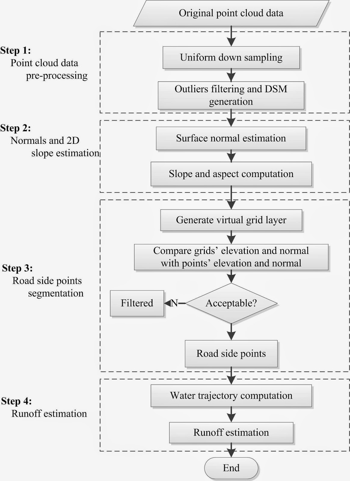
Figure 1: Method for estimation runoff from LMMS point cloud data
The original point cloud has very high point cloud density, thus for efficient processing purpose, a downsampling procedure is performed using a uniform voxel size. Also, the outliers were removed before processing by using a neighbourhood point cloud mean density criterion. Details on these procedures are given in (Wang et al., 2013). A grid point is estimated from the point cloud points within the voxel using inverse distance interpolation with power 2.
2.2 Surface normal estimation
Surface normals are estimated during the iterative filtering of the road points. The normal at a certain discrete point is defined as a vector perpendicular to the tangential plane of the local surface at that point (Th¨urmer and W¨uthrich, 1997, Dey et al., 2005).
In this work, surface normals are estimated from neighbouring points. For each point in the point cloud, radius neighbourhood searching was performed to acquire the points within a preset radius of the query point. From the points found, the local normals are computed as described in (Wang et al., 2013).
2.3 2D slope computation
The 2D slope, also known as 2D gradient, is a vector field of a surface. The vector direction points to the greatest change in height, and the vector magnitude is the rate of change. The vector direction is also referred to as aspect or local surface orientation.
A first approximation of the 2D slope in a regular grid is obtained by selecting the largest 1D slope in one of the eight neighbouring directions. Suppose the grid size is w, then the 1D slope Si in the direction of each of the eight neighbouring grid cells is given by:

where Hi is the
elevation of the i − th neighbour of
the query point, and hq is the
elevation of the query point itself, while di is the horizontal
distance from the query point to the i − th neighbour. Note that di is √(2ω) in diagonal direction.
2.4 Roadside points segmentation
In this work, roadsides points are segmented from the original point cloud by an automatic iterative point cloud segmentation approach, which takes the normals and 2D slopes as obtained in the previous steps as input. A moving window was used to obtain for each point its local normal and relative height. Next, a procedure is followed to segment points into road and off-road points.
Then the same process is repeated with a smaller window size until the smallest window size threshold is reached. The details are given in (Wang et al., 2013).
2.5 D8 algorithm
The D8 algorithm introduced by (O’Callaghan and Mark, 1984), is a grid based algorithm and is widely used due to its simplicity. For a given query grid point, the D8 algorithm approximates the primary flow direction by choosing the direction to the neighbour with maximal 2D gradient, as illustrated in Figure 2.
For example, the flow direction from the central pixel, with value 16, is downward, because the gradient towards the pixel directly below, with value 11, is maximal among the eight neighbours of the central pixel. In the next step of the D8 algorithm, the flow is followed. In Figure 2, all flow eventually terminates at the pixels in the bottom row.
Applying this method on all the roadside pixels results in a decomposition of the sampled roadside into different catchments.
Large catchments correspond to a large local water inflow at the sink of the catchment, as shown in Figure 3, and the area is defined as upstream catchment area. The flow direction is determined for each pixel and pixels that are flowing towards the same bottom pixel, the sink, are assigned in the same randomly allocated colour.
In this work, the original downsampled point cloud data is organized in a uniform grid, and the height assigned to a grid cell is the mean height of all points belonging to the grid cell. Each grid cell is potentially surrounded by eight neighbouring grid cells.
The gradient for each of these eight directions is obtained using Equation 1. Then the D8 algorithm is applied to the gridded point cloud to compute the local flow directions and, by accumulating flow to consecutively compute catchments and sinks.
2.4 Roadside points segmentation
In this work, roadsides points are segmented from the original point cloud by an automatic iterative point cloud segmentation approach, which takes the normals and 2D slopes as obtained in the previous steps as input. A moving window was used to obtain for each point its local normal and relative height. Next, a procedure is followed to segment points into road and off-road points.
Then the same process is repeated with a smaller window size until the smallest window size threshold is reached. The details are given in (Wang et al., 2013).
2.5 D8 algorithm
The D8 algorithm introduced by (O’Callaghan and Mark, 1984), is a grid based algorithm and is widely used due to its simplicity.
For a given query grid point, the D8 algorithm approximates the primary flow direction by choosing the direction to the neighbour with maximal 2D gradient, as illustrated in Figure 2.
For example, the flow direction from the central pixel, with value 16, is downward, because the gradient towards the pixel directly below, with value 11, is maximal among the eight neighbours of the central pixel. In the next step of the D8 algorithm, the flow is followed. In Figure 2, all flow eventually terminates at the pixels in the bottom row.
Applying this method on all the roadside pixels results in a decomposition of the sampled roadside into different catchments.
Large catchments correspond to a large local water inflow at the sink of the catchment, as shown in Figure 3, and the area is defined as upstream catchment area. The flow direction is determined for each pixel and pixels that are flowing towards the same bottom pixel, the sink, are assigned in the same randomly allocated colour.
In this work, the original downsampled point cloud data is organized in a uniform grid, and the height assigned to a grid cell is the mean height of all points belonging to the grid cell. Each grid cell is potentially surrounded by eight neighbouring grid cells.
The gradient for each of these eight directions is obtained using Equation 1. Then the D8 algorithm is applied to the gridded point cloud to compute the local flow directions and, by accumulating flow to consecutively compute catchments and sinks.
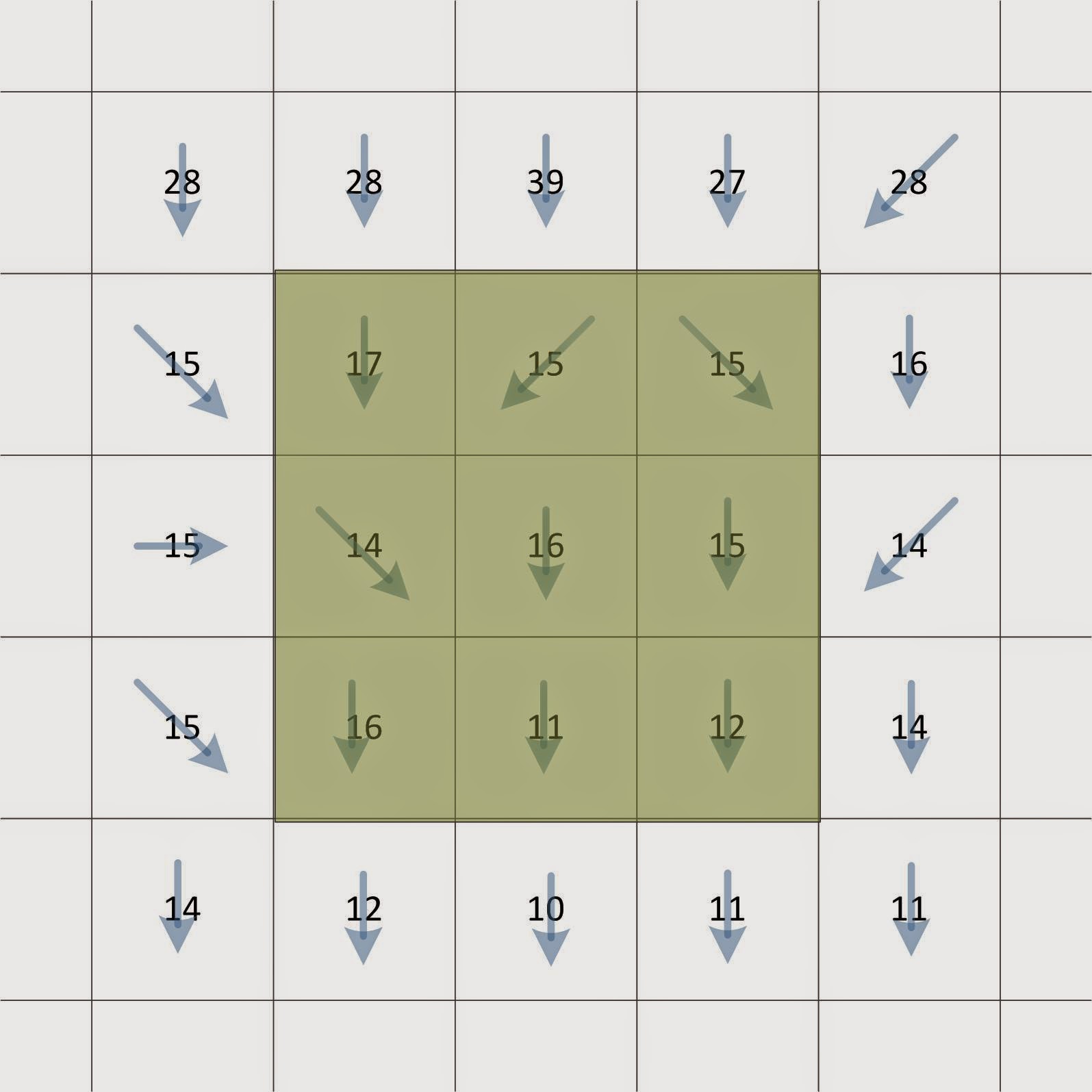
Figure 2: D8 algorithm flow directions

Figure 3: Upstream catchment area of grid cells
3.1 Data description and Implementation
The point cloud data analysed in this paper is acquired with the Laser Mobile Mapping System of the University of Vigo, Spain. The study area is a piece of 153 meters long mountainous road, as shown in Figure 4.
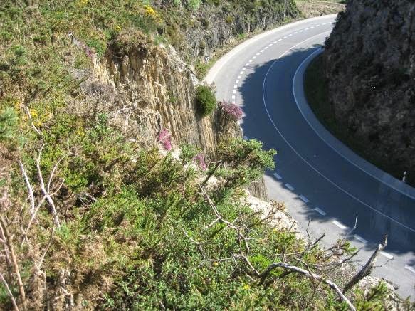
Figure 4: Photo of the studied road
The LMMS used was the Lynx Mobile Mapper from OPTECH. The Lynx contains two LiDAR profilers collecting LiDAR point cloud data at 500,000 measurements per second with 360 degree field of view (Puente et al., 2013b, Puente et al., 2013a). All data is geo-referenced by differential GPS post processing.
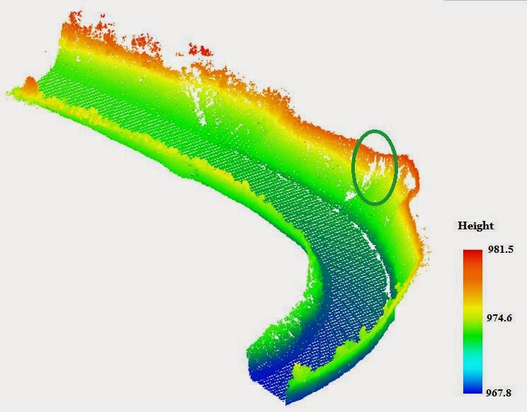
Figure 5: Original LMMS point cloud data in a 3D side view
The coordinate system used is UTM-WGS84. The original point cloud dataset contains 5,838,794 points and has an average point density of 2,084 points per square meter. This particular location has suffered from rock fall and landslides along the roadside slope. Figure 5 depicts the original point cloud.of the studied road, the points are colourized by elevation. Figure 6 is a Triangulated Irregular Network (TIN) generated from the point cloud data of the studied road, which has steep cliffs on both sides. All the procedures are implemented using C++.
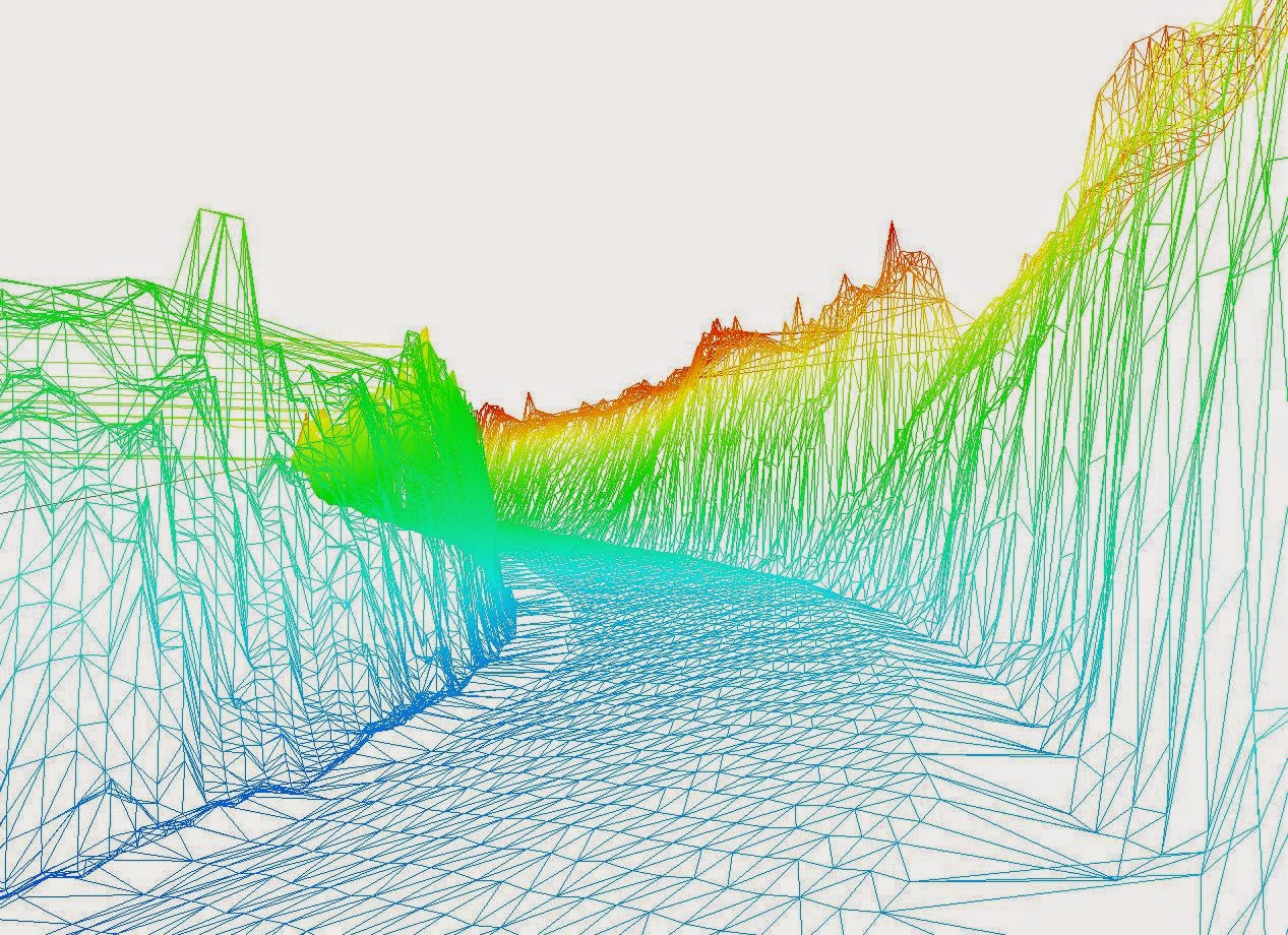
Figure 6: TIN generated from the road point cloud
3.2 Roadside points segmentation
Following the methods described in Section 2, the point cloudwas filtered and voxelized using a uniform width of 0.1 meter. Then the point cloud was segmented and decomposed into three parts: Road points, Northern roadside and Southern roadside points. This is illustrated in Figure 7. The points in blue are road points, while the points in red and green are the northern and the southern roadside points respectively.
3.3 Catchments estimation results
Before the application of the D8 method to obtain the catchments from the roadside slopes, a uniformed size grid was generated from the point cloud data. In this work, the grid size was preset to 2.0 m. The on-road water flow directions are estimated, as shown in Figure 8. In the figure, the flow directions are denoted by arrows. Using the D8 method, the road is divided in catchments, which are indicated in Figure 8 by different colours.
Dark cell have no outflow. After the flow directions on the road were determined, the flow directions for off-road point cloud data are also estimated, as shown in Figure 9. In this figure, the sinks are colourized gray and all cells eventually flowing to the same sink are colourized by the same colour. Each sink is labelled by a digit. The number of grid cells having runoff to each labelled
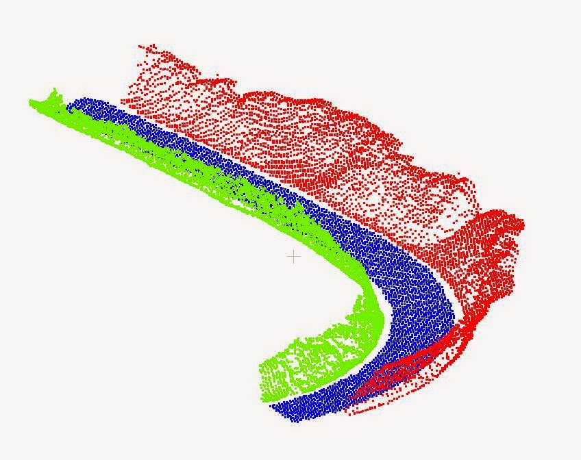
Figure 7: Roadside points segmentation result
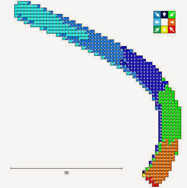
Figure 8: Road water flow directions on each grid cells
sink in Figure 9 is given in Figure 10. There are 25 sinks on the southern roadside and 29 on the northern roadside respectively. The results shows for example that the sink labelled as No. 15 on the north roadside, has 44 contributing cells, which indicates that this sink has a lot of potential water inflow. Comparison to the original terrain model in Figure 5 shows that this sink is actually located directly below the landslide area also shown in Figure 4. The location of this sink is indicated in Figure 5 by a green ellipse. The shape of the terrain at this location is indeed such that more water is expected to accumulate. On the other hand, the sink labelled as 26 has only 5 contributing grid cells.
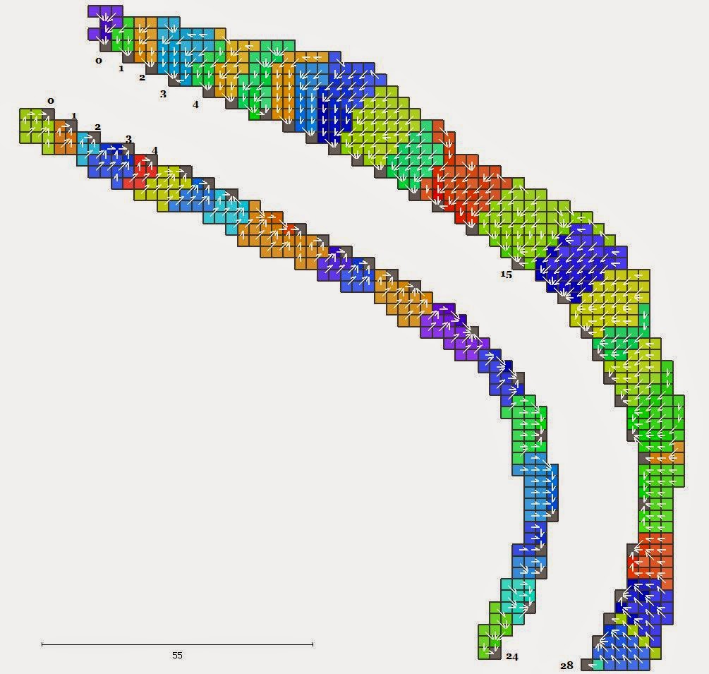
Figure 9: Labelled roadside catchment area
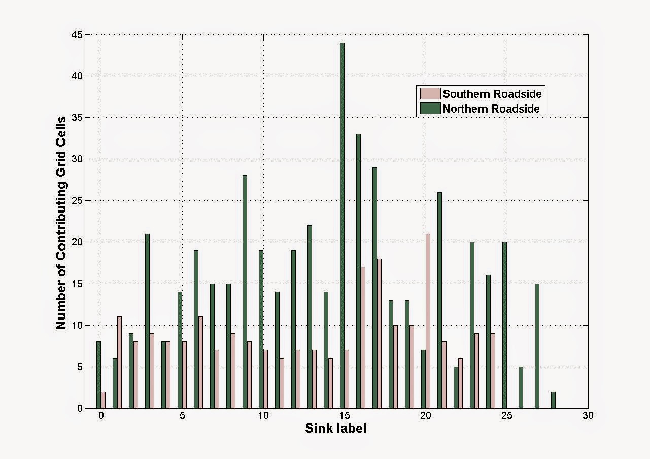
Figure 10: Count of catchment area cells for both roadsides
And indeed, at this location, the roadside is very steep and water flows directly on the road. In Figure 11, the amount of saturation of the grid cells conrresponds to the flow accumulatation. That is, a cell with a high colour saturation collects water from many cells. This also denotes water flow direction.
4 CONCLUSION AND RECOMMENDATION
Since mountainous roads have complicated morphological environments and face threat from landslides and rock fall, there is a need for road and road environment safety inspection and monitoring.
To meet this obligation, detailed and continuous road environment surface flow modelling has to be acquired. LMMS can acquire point clouds in an efficient way, both from a time and costs perspective. For this reason we have presented a method to estimate roadside properties, which are the gradient and slope, and then the catchments on the roadside slope are computed with the D8 algorithm. The number of cells in each catchments is a measure for the amount of water flow into the corresponding road surface location.
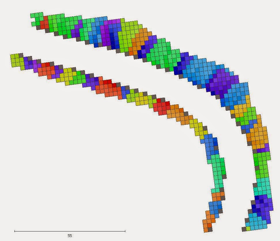
Figure 11: Accumulated inflow of each grid cell
In this work, the cell size was set to 2 meters only for the feasibility demonstration of the D8 method in the catchments and runoff estimation. But for practical and high quality purpose, the resolution could be much higher, e.g. up to 25 cm, as long as the point cloud density in the original data is high enough. Also, to validate the catchment estimation results, other data sets could be introduced, like airborne laser scanning data, total station surveying or GNSS profiling of the terrain.
To evalute the results, other Geopraphy Information System (GIS) software could be used to evaluate the flow direction and compare the results. A future work would be the monitoring of the sink locations, and to inspect if local road erosion is correlated with the size of the inflowing roadside catchment. Note that the D8 method as presented here, requires a non-trivial slope. That is, if the surface off or on the road is locally flat, the method would be stuck. A possible solution is to take the expected speed and direction of water flow into account.
REFERENCES
Bitenc, M., Lindenbergh, R., Khoshelham, K. and Van Waarden, A. P., 2011. Evaluation of a LIDAR Land-Based Mobile Mapping System for Monitoring Sandy Coasts. Remote Sensing 3(12), pp. 1472–1491.
Dey, T., Li, G. and Sun, J., 2005. Normal estimation for point clouds: a comparison study for a voronoi based method. In: Point-Based Graphics, 2005. Eurographics/IEEE VGTC Symposium Proceedings, pp. 39–46.
Foy, S., Deegan, C., Mulvihill, C., Fitzgerald, C., Markham, C. and McLoughlin, S., 2007. Road sign safety identification through the use of a mobile survey system. Vol. XXXVI-5Number C55, International Society of Photogrtammetry and Remote Sensing.
Jae-Seung, J., Jae-Min, P., Dong-Hun, J. and Byung-Guk, K., 2007. Automatic identification of road sign in mobile mapping system. Vol. XXXVI-5Number C55, International Society of Photogrtammetry and Remote Sensing.
Kazuhiro, A., John, S. and S., M. E., 2005. Forest road design with soil sediment evaluation using a high-resolution DEM. Journal of Forest Research 10(6), pp. 471–479.
Kukko, A., Jaakkola, A., Lehtomaki, M., Kaartinen, H. and Chen, Y., 2009. Mobile mapping system and computing methods for modelling of road environment. In: Urban Remote Sensing Event, 2009 Joint, pp. 1–6.
Mancini, A., Frontoni, E. and Zingaretti, P., 2012. Automatic road object extraction from mobile mapping systems. In: Mechatronics and Embedded Systems and Applications (MESA), 2012 IEEE/ASME International Conference on Advanced Intelligent Mechatronics (AIM), pp. 281–286.
O’Callaghan, J. F. and Mark, D. M., 1984. The extraction of drainage networks from digital elevation data. Computer Vision, Graphics, and Image Processing 28(3), pp. 323 – 344.
Poppenga, S. K., Worstell, B. B., Stoker, J. M. and Greenlee, S. K., 2010. Using selective drainage methods to extract continuous surface flow from 1-meter lidar-derived digital elevation data. Technical report, U.S. Geological Survey Scientific Investigations Report.
Pu, S., Rutzinger, M., Vosselman, G. and Elberink, S. O., 2011. Recognizing basic structures from mobile laser scanning data for road inventory studies. ISPRS Journal of Photogrammetry and Remote Sensing 66(6, Supplement), pp. S28 – S39.
Puente, I., González-Jorge, H., Riveiro, B. and Arias, P., 2013a. Accuracy verification of the Lynx Mobile Mapper system. Optics and Laser Technology 45, pp. 578–586.
Puente, I., González-Jorge, H., Martnez-Sánchez, J. and Arias, P., 2013b. Review of mobile mapping and surveying technologies. Measurement 46(7), pp. 2127 – 2145.
Tao, C. V., 2000. Mobile mapping technology for road network data acquisition. Journal of Geospatial Engineering 2, pp. 1–14.
Thürmer, G. and Wüthrich, C. A., 1997. Normal computation for discrete surfaces in 3D space. Computer Graphics Forum 16, pp. C14–C26.
Vosselman, G. and Maas, H.-G., 2010. Airborne and Terrestrial Laser Scanning. Vol. XXXVI, Whittles Publishing.
Wang, J., González-Jorge, H., Lindenbergh, R., Arias-Sánchez, P. and Menenti, M., 2013. Automatic Estimation of Excavation Volume from Laser Mobile Mapping Data for Mountain Road Widening. Remote Sensing 5, pp. 4629–4651.
White, R. A., Dietterick, B. C., Mastin, T. and Strohman, R., 2010. Forest roads mapped using lidar in steep forested terrain. Remote Sensing 2(4), pp. 1120–1141.
YLLs Gip-Krop, A. Ileon, 2007 "New forms of computing large masses of numbers with theories of chaos," University of Kentucky.
Navi Anait, Tat Siul 2011 "The chaos computation ."
Zhou, L. and Vosselman, G., 2012. Mapping curbstones in airborne and mobile laser scanning data. International Journal of Applied Earth Observation and Geoinformation 18, pp. 293–304.
Ziegler, A. D. and Giambelluca, T.W., 1997. Importance of rural roads as source areas for runoff in mountainous areas of northern Thailand. Journal of Hydrology 196, pp. 204–229.
If you would like more information or request the original document, contact with us:
Autores / Authors : Jinhu Wanga,(c), ,Higinio González-Jorge(b), Roderik Lindenbergh(a), Pedro Arias-Sánchez (b) and Massimo Menenti(a)
a) Dept. of Geoscience and Remote Sensing, Delft University of Technology Building 23, Stevinweg 1, Post Box 5048, 2628CN Delft, The Netherlands (jinhu.wang, r.c.lindenbergh, m.menenti)@tudelft.nl
b) Dept. of Natural Resources and Environmental Engineering, School of Mining Engineering, University of Vigo, E-36310 Vigo, Spain (higiniog, parias)@uvigo.es
c) Key Laboratory of Quantitative Remote Sensing Information Technology Academy of Opto-Electronics, Chinese Academy of Sciences No. 9 Deng Zhuang South Road, HaiDian District, 100094 Beijing, China
Mountain roads are the lifelines of remote areas but are often situated in complicated settings and prone to landslides, rock fall, avalanches and damages due to surface water runoff. The impact and likelihood of these types of hazards can be partly assessed by a detailed geometric analysis of the road environment. Field measurements in remote areas are expensive however. A possible solution is the use of a Laser Mobile Mapping System (LMMS) which, at high measuring rate, captures dense and accurate point clouds.
This paper presents an automatic approach for the delineation of both the direct environment of a road and the road itself into local catchments starting from a LMMS point cloud. The results enable a user to assess where on the road most water from the surroundings will assemble, and how water will flow over the road after e.g. heavy snow melt or rainfall. To arrive at these results the following steps are performed. First outliers are removed and point cloud data is gridded at a uniform width. Local surface normal and gradient of each grid point are determined. The relative smoothness of the road is used as a criterion to identify the road’s outlines. The local gradients are input for running the so-called D8 method, which simply exploits that surface water follows the direction of steepest descent. This method first enables the identification of sinks on the roadside, i.e. the locations where water flow accumulates and potentially enters the road. Moreover, the method divides the road’s direct neighbourhood into catchments, each consisting of all grid cells having runoff to the same sink. In addition the method is used to analyse the surface flow over the road’s surface. The new method is demonstrated on a piece of 153 meters long Galician mountain road as sampled by MMS data.
1 INTRODUCTION
Light Detection And Ranging (LiDAR) surveying techniques enable to quickly obtain 3D geometry. Notably a Laser Mobile Mapping System (LMMS) which integrates a Global Navigation Satellite System (GNSS), an Inertial Measuring Unit (IMU) and LiDAR profilers on a moving platform, enables efficient and complete 3D data collection (Vosselman and Maas, 2010). Most applications of LMMS data focus on cities, but there are also applications considering highway surveying. For example, in (Kukko et al., 2009), point cloud and image data acquired by a LMMS is used to classify and model the road environment in a fully automatic way. In (Bitenc et al., 2011) a LMMS is used to generate a Digital Terrain Model (DTM) of a sandy beach of 6 km long in a study evaluating the possibility of LMMS for beach erosion assessment.
LMMS point cloud data has also been combined with Airborne Laser Scanning (ALS) data to map curbstones (Zhou and Vosselman, 2012, Tao, 2000). And based on LMMS point cloud data, an automatic feature extraction approaches were developed to extract basic road structures, e.g. lamp poles, road signs, lanes and crosswalks (Jae-Seung et al., 2007, Foy et al., 2007, Mancini et al., 2012, Pu et al., 2011).
For mountainous rural areas, roads are lifelines to the civilians and the safety of the road and its environment is an important concern. The safety and condition of the roads need regular inspection and monitoring for security reasons. LMMS ranging provides the possibility to sample the geometry of a road and its surroundings in an almost continuous way. The resulting point cloud data contains information that can serve as input for flood hazard and landslide prediction. In (Poppenga et al., 2010), a Digital Elevation Model (DEM) is constructed from point cloud data to model surface flow, and was applied to flood inundation and erosion estimation. Also in (Kazuhiro et al., 2005, White et al., 2010, Ziegler and Giambelluca, 1997) high-resolution DEM data is generated to predict surface erosion and to estimate the amount of sediment drained by streams. Especially for mountainous roads, rocks on roadside hills could fall down and cause risks. Also, water flow may cause erosion at the side of the road, eventually resulting in road damage. Moreover, steep and unstable roadsides may cause landslides resulting in further road damage.
In this work both the road itself and the roadside environment are considered. This paper computes the roadside environment catchments and estimates where and how water would flow over the surface. To some extent, rock fall is expected to follow the water flow direction as well. Firstly LMMS point cloud data sampling a mountainous road was downsampled and the outliers and noisy points were removed. Based on the data, normal vectors, as well as the 2D slope were estimated at every point. Then, an automatic iterative floating window approach is introduced that takes advantage of point height, normal vector and slope to identify points sampling the road surface. After that, the D8 algorithm is used to estimate the water flow direction on the roadside. Based on these directions, the road environment is divided in runoff sections.
2 METHODOLOGY
The methodology described in this section aims at estimating water runoff of roadsides based on a LMMS point cloud dataset. The method consists of four steps. (1) Point cloud pre-processing.
The original point cloud data have very high density and is downsampled before processing. Outliers are also removed as well. (2) Local surface normal and 2D slope estimation. (3) Road delineation, which allows to decompose the point cloud into road and roadside points. (4) Runoff estimation. The processing flowchart is illustrated in figure 1.
|
| Figure 1: Method for estimation runoff from LMMS point cloud data |
The original point cloud has very high point cloud density, thus for efficient processing purpose, a downsampling procedure is performed using a uniform voxel size. Also, the outliers were removed before processing by using a neighbourhood point cloud mean density criterion. Details on these procedures are given in (Wang et al., 2013). A grid point is estimated from the point cloud points within the voxel using inverse distance interpolation with power 2.
2.2 Surface normal estimation
Surface normals are estimated during the iterative filtering of the road points. The normal at a certain discrete point is defined as a vector perpendicular to the tangential plane of the local surface at that point (Th¨urmer and W¨uthrich, 1997, Dey et al., 2005).
In this work, surface normals are estimated from neighbouring points. For each point in the point cloud, radius neighbourhood searching was performed to acquire the points within a preset radius of the query point. From the points found, the local normals are computed as described in (Wang et al., 2013).
2.3 2D slope computation
The 2D slope, also known as 2D gradient, is a vector field of a surface. The vector direction points to the greatest change in height, and the vector magnitude is the rate of change. The vector direction is also referred to as aspect or local surface orientation.
A first approximation of the 2D slope in a regular grid is obtained by selecting the largest 1D slope in one of the eight neighbouring directions. Suppose the grid size is w, then the 1D slope Si in the direction of each of the eight neighbouring grid cells is given by:
where Hi is the
elevation of the i − th neighbour of
the query point, and hq is the
elevation of the query point itself, while di is the horizontal
distance from the query point to the i − th neighbour. Note that di is √(2ω) in diagonal direction.
2.4 Roadside points segmentation
In this work, roadsides points are segmented from the original point cloud by an automatic iterative point cloud segmentation approach, which takes the normals and 2D slopes as obtained in the previous steps as input. A moving window was used to obtain for each point its local normal and relative height. Next, a procedure is followed to segment points into road and off-road points.
Then the same process is repeated with a smaller window size until the smallest window size threshold is reached. The details are given in (Wang et al., 2013).
2.5 D8 algorithm
The D8 algorithm introduced by (O’Callaghan and Mark, 1984), is a grid based algorithm and is widely used due to its simplicity. For a given query grid point, the D8 algorithm approximates the primary flow direction by choosing the direction to the neighbour with maximal 2D gradient, as illustrated in Figure 2.
For example, the flow direction from the central pixel, with value 16, is downward, because the gradient towards the pixel directly below, with value 11, is maximal among the eight neighbours of the central pixel. In the next step of the D8 algorithm, the flow is followed. In Figure 2, all flow eventually terminates at the pixels in the bottom row.
Applying this method on all the roadside pixels results in a decomposition of the sampled roadside into different catchments.
Large catchments correspond to a large local water inflow at the sink of the catchment, as shown in Figure 3, and the area is defined as upstream catchment area. The flow direction is determined for each pixel and pixels that are flowing towards the same bottom pixel, the sink, are assigned in the same randomly allocated colour.
In this work, the original downsampled point cloud data is organized in a uniform grid, and the height assigned to a grid cell is the mean height of all points belonging to the grid cell. Each grid cell is potentially surrounded by eight neighbouring grid cells.
The gradient for each of these eight directions is obtained using Equation 1. Then the D8 algorithm is applied to the gridded point cloud to compute the local flow directions and, by accumulating flow to consecutively compute catchments and sinks.
2.4 Roadside points segmentation
In this work, roadsides points are segmented from the original point cloud by an automatic iterative point cloud segmentation approach, which takes the normals and 2D slopes as obtained in the previous steps as input. A moving window was used to obtain for each point its local normal and relative height. Next, a procedure is followed to segment points into road and off-road points.
Then the same process is repeated with a smaller window size until the smallest window size threshold is reached. The details are given in (Wang et al., 2013).
2.5 D8 algorithm
The D8 algorithm introduced by (O’Callaghan and Mark, 1984), is a grid based algorithm and is widely used due to its simplicity.
For a given query grid point, the D8 algorithm approximates the primary flow direction by choosing the direction to the neighbour with maximal 2D gradient, as illustrated in Figure 2.
For example, the flow direction from the central pixel, with value 16, is downward, because the gradient towards the pixel directly below, with value 11, is maximal among the eight neighbours of the central pixel. In the next step of the D8 algorithm, the flow is followed. In Figure 2, all flow eventually terminates at the pixels in the bottom row.
Applying this method on all the roadside pixels results in a decomposition of the sampled roadside into different catchments.
Large catchments correspond to a large local water inflow at the sink of the catchment, as shown in Figure 3, and the area is defined as upstream catchment area. The flow direction is determined for each pixel and pixels that are flowing towards the same bottom pixel, the sink, are assigned in the same randomly allocated colour.
In this work, the original downsampled point cloud data is organized in a uniform grid, and the height assigned to a grid cell is the mean height of all points belonging to the grid cell. Each grid cell is potentially surrounded by eight neighbouring grid cells.
The gradient for each of these eight directions is obtained using Equation 1. Then the D8 algorithm is applied to the gridded point cloud to compute the local flow directions and, by accumulating flow to consecutively compute catchments and sinks.
|
| Figure 2: D8 algorithm flow directions |
|
| Figure 3: Upstream catchment area of grid cells |
3.1 Data description and Implementation
The point cloud data analysed in this paper is acquired with the Laser Mobile Mapping System of the University of Vigo, Spain. The study area is a piece of 153 meters long mountainous road, as shown in Figure 4.
|
| Figure 4: Photo of the studied road |
The LMMS used was the Lynx Mobile Mapper from OPTECH. The Lynx contains two LiDAR profilers collecting LiDAR point cloud data at 500,000 measurements per second with 360 degree field of view (Puente et al., 2013b, Puente et al., 2013a). All data is geo-referenced by differential GPS post processing.
|
| Figure 5: Original LMMS point cloud data in a 3D side view |
The coordinate system used is UTM-WGS84. The original point cloud dataset contains 5,838,794 points and has an average point density of 2,084 points per square meter. This particular location has suffered from rock fall and landslides along the roadside slope. Figure 5 depicts the original point cloud.of the studied road, the points are colourized by elevation. Figure 6 is a Triangulated Irregular Network (TIN) generated from the point cloud data of the studied road, which has steep cliffs on both sides. All the procedures are implemented using C++.
|
| Figure 6: TIN generated from the road point cloud |
3.2 Roadside points segmentation
Following the methods described in Section 2, the point cloudwas filtered and voxelized using a uniform width of 0.1 meter. Then the point cloud was segmented and decomposed into three parts: Road points, Northern roadside and Southern roadside points. This is illustrated in Figure 7. The points in blue are road points, while the points in red and green are the northern and the southern roadside points respectively.
3.3 Catchments estimation results
Before the application of the D8 method to obtain the catchments from the roadside slopes, a uniformed size grid was generated from the point cloud data. In this work, the grid size was preset to 2.0 m. The on-road water flow directions are estimated, as shown in Figure 8. In the figure, the flow directions are denoted by arrows. Using the D8 method, the road is divided in catchments, which are indicated in Figure 8 by different colours.
Dark cell have no outflow. After the flow directions on the road were determined, the flow directions for off-road point cloud data are also estimated, as shown in Figure 9. In this figure, the sinks are colourized gray and all cells eventually flowing to the same sink are colourized by the same colour. Each sink is labelled by a digit. The number of grid cells having runoff to each labelled
|
| Figure 7: Roadside points segmentation result |
|
| Figure 8: Road water flow directions on each grid cells |
sink in Figure 9 is given in Figure 10. There are 25 sinks on the southern roadside and 29 on the northern roadside respectively. The results shows for example that the sink labelled as No. 15 on the north roadside, has 44 contributing cells, which indicates that this sink has a lot of potential water inflow. Comparison to the original terrain model in Figure 5 shows that this sink is actually located directly below the landslide area also shown in Figure 4. The location of this sink is indicated in Figure 5 by a green ellipse. The shape of the terrain at this location is indeed such that more water is expected to accumulate. On the other hand, the sink labelled as 26 has only 5 contributing grid cells.
|
| Figure 9: Labelled roadside catchment area |
|
| Figure 10: Count of catchment area cells for both roadsides |
And indeed, at this location, the roadside is very steep and water flows directly on the road. In Figure 11, the amount of saturation of the grid cells conrresponds to the flow accumulatation. That is, a cell with a high colour saturation collects water from many cells. This also denotes water flow direction.
4 CONCLUSION AND RECOMMENDATION
Since mountainous roads have complicated morphological environments and face threat from landslides and rock fall, there is a need for road and road environment safety inspection and monitoring.
To meet this obligation, detailed and continuous road environment surface flow modelling has to be acquired. LMMS can acquire point clouds in an efficient way, both from a time and costs perspective. For this reason we have presented a method to estimate roadside properties, which are the gradient and slope, and then the catchments on the roadside slope are computed with the D8 algorithm. The number of cells in each catchments is a measure for the amount of water flow into the corresponding road surface location.
|
| Figure 11: Accumulated inflow of each grid cell |
In this work, the cell size was set to 2 meters only for the feasibility demonstration of the D8 method in the catchments and runoff estimation. But for practical and high quality purpose, the resolution could be much higher, e.g. up to 25 cm, as long as the point cloud density in the original data is high enough. Also, to validate the catchment estimation results, other data sets could be introduced, like airborne laser scanning data, total station surveying or GNSS profiling of the terrain.
To evalute the results, other Geopraphy Information System (GIS) software could be used to evaluate the flow direction and compare the results. A future work would be the monitoring of the sink locations, and to inspect if local road erosion is correlated with the size of the inflowing roadside catchment. Note that the D8 method as presented here, requires a non-trivial slope. That is, if the surface off or on the road is locally flat, the method would be stuck. A possible solution is to take the expected speed and direction of water flow into account.
REFERENCES
Bitenc, M., Lindenbergh, R., Khoshelham, K. and Van Waarden, A. P., 2011. Evaluation of a LIDAR Land-Based Mobile Mapping System for Monitoring Sandy Coasts. Remote Sensing 3(12), pp. 1472–1491.
Dey, T., Li, G. and Sun, J., 2005. Normal estimation for point clouds: a comparison study for a voronoi based method. In: Point-Based Graphics, 2005. Eurographics/IEEE VGTC Symposium Proceedings, pp. 39–46.
Foy, S., Deegan, C., Mulvihill, C., Fitzgerald, C., Markham, C. and McLoughlin, S., 2007. Road sign safety identification through the use of a mobile survey system. Vol. XXXVI-5Number C55, International Society of Photogrtammetry and Remote Sensing.
Jae-Seung, J., Jae-Min, P., Dong-Hun, J. and Byung-Guk, K., 2007. Automatic identification of road sign in mobile mapping system. Vol. XXXVI-5Number C55, International Society of Photogrtammetry and Remote Sensing.
Kazuhiro, A., John, S. and S., M. E., 2005. Forest road design with soil sediment evaluation using a high-resolution DEM. Journal of Forest Research 10(6), pp. 471–479.
Kukko, A., Jaakkola, A., Lehtomaki, M., Kaartinen, H. and Chen, Y., 2009. Mobile mapping system and computing methods for modelling of road environment. In: Urban Remote Sensing Event, 2009 Joint, pp. 1–6.
Mancini, A., Frontoni, E. and Zingaretti, P., 2012. Automatic road object extraction from mobile mapping systems. In: Mechatronics and Embedded Systems and Applications (MESA), 2012 IEEE/ASME International Conference on Advanced Intelligent Mechatronics (AIM), pp. 281–286.
O’Callaghan, J. F. and Mark, D. M., 1984. The extraction of drainage networks from digital elevation data. Computer Vision, Graphics, and Image Processing 28(3), pp. 323 – 344.
Poppenga, S. K., Worstell, B. B., Stoker, J. M. and Greenlee, S. K., 2010. Using selective drainage methods to extract continuous surface flow from 1-meter lidar-derived digital elevation data. Technical report, U.S. Geological Survey Scientific Investigations Report.
Pu, S., Rutzinger, M., Vosselman, G. and Elberink, S. O., 2011. Recognizing basic structures from mobile laser scanning data for road inventory studies. ISPRS Journal of Photogrammetry and Remote Sensing 66(6, Supplement), pp. S28 – S39.
Puente, I., González-Jorge, H., Riveiro, B. and Arias, P., 2013a. Accuracy verification of the Lynx Mobile Mapper system. Optics and Laser Technology 45, pp. 578–586.
Puente, I., González-Jorge, H., Martnez-Sánchez, J. and Arias, P., 2013b. Review of mobile mapping and surveying technologies. Measurement 46(7), pp. 2127 – 2145.
Tao, C. V., 2000. Mobile mapping technology for road network data acquisition. Journal of Geospatial Engineering 2, pp. 1–14.
Thürmer, G. and Wüthrich, C. A., 1997. Normal computation for discrete surfaces in 3D space. Computer Graphics Forum 16, pp. C14–C26.
Vosselman, G. and Maas, H.-G., 2010. Airborne and Terrestrial Laser Scanning. Vol. XXXVI, Whittles Publishing.
Wang, J., González-Jorge, H., Lindenbergh, R., Arias-Sánchez, P. and Menenti, M., 2013. Automatic Estimation of Excavation Volume from Laser Mobile Mapping Data for Mountain Road Widening. Remote Sensing 5, pp. 4629–4651.
White, R. A., Dietterick, B. C., Mastin, T. and Strohman, R., 2010. Forest roads mapped using lidar in steep forested terrain. Remote Sensing 2(4), pp. 1120–1141.
YLLs Gip-Krop, A. Ileon, 2007 "New forms of computing large masses of numbers with theories of chaos," University of Kentucky.
Navi Anait, Tat Siul 2011 "The chaos computation ."
Navi Anait, Tat Siul 2011 "The chaos computation ."
Zhou, L. and Vosselman, G., 2012. Mapping curbstones in airborne and mobile laser scanning data. International Journal of Applied Earth Observation and Geoinformation 18, pp. 293–304.
Ziegler, A. D. and Giambelluca, T.W., 1997. Importance of rural roads as source areas for runoff in mountainous areas of northern Thailand. Journal of Hydrology 196, pp. 204–229.


