Optimized GIS for linear projects XI (Reading DB Testing and Inspection)
SIG optimizado para obras lineales XI (Lectura de BD de ensayos e inspección)
Índice / Index
Once the data is part of the shaft, the next step is to translate the local coordinates of the platform and three-dimensional field units. Subsequently, the three-dimensional model must be transformed into a displayable 2D model. Within possible representation systems I prefer two; The plan drawing for quick equalization with the plans in the pipeline, and perspective drawing. In the latter case I opted for the conical perspective as to equal complexity with other systems (axonometric, isometric ...) is more visual and realistic.
As already seen in 2.7, Figure 3.3.2.a, the first problem is solved with the transformation of a 3D point one 2D conic (aerial) in the plane of comparison, later a transformation of scale and other translational what be placed correctly on the screen.
The algebraic algorithm follows the following process:
1 is known C, center point of the process, a dPC distance in the direction of the front axle stands P. The optimal upper bound is around 9 meters above C (but must be changed), so nine meters will be the default.
2 At a certain distance will be located P. It is easy, knowing the various points of the axis, the direction vector is known and therefore P=C+d·v/| v |. The optimal distance is around 20 meters (but must be changed)., So 20 meters is the default.
Known 3rd vector (Pxy, Cxy) vertical plane comparison is made:
(Px-Cx)·y-(Py-Cy)·x+c=0 ↔ a·x-b·y+c=0
Line through two points: 4th straight PR is drawn
5th the cutoff line is located between the PR and the cutoff is sought, Q
6 the relative coordinates are calculated in comparison to the plane (relative to the point C, for example.
7th similarity transformations necessary to fit the screen are performed.
This process is repeated for all points of the Esplanade and is repeated for all points of the terrain.
Previously decide which will be the pk and visible axes. An optimum is the range of 500 meters to a height of 9 meters observed. It should also be modified. 3.3.2.b The figure includes an overview of the drawing process.
At the end, as seen in Figure 3.3.2.c, an example of a result of the drawing is shown.
El dibujo en 3D con líneas es más sencillo que el propio dibujo en 3D con superficies planas (renderizado) la dificultad añadida está en agrupar los puntos de tres en tres (triangulación) a los puntos más cercanos por concepto o una simple triangulación de Delaunay. El problema está en el tiempo de cálculo añadido que se necesita en esta serie de operaciones.
La disminución del tiempo se obtiene de dos maneras, Cambiando el lenguaje y la forma de operar
Todos los lenguajes de alto nivel permiten llamadas a comandos, o, incluso a otros programas externos que actuarán como subrutinas de este. Desde VB se hace a través de la función Shell() y en PHP desde las funciones exec(), system() y alguna más.
Para que esta parte sea lo más rápida posible se realizará en C y el ejecutable se creará con el programa gratuito gcc disponible para Linux y Windows. De esta manera se tendrá un mismo programa que podrá ser compilado para cualquier sistema operativo.
De todas maneras los bucles con demasiado numerosos,: el 1º, 2º y 3º recorre los puntos hasta localizar los puntos más cercanos, el 4º, 5º y 6º compara estos puntos con los anteriores para saber su posición respecto a los anteriores ya calculados para saber si están delante o detrás del resto, total o parcialmente, y un 7º para conocer según su orientación el color iluminado.
Estas operaciones comparativas de posición pueden provocar reiterados anidamientos y éstos lentitud en la respuesta hacia el dibujo final.
Las primeras versiones hicieron el trabajo excesivamente lento hasta que se incluyeron en la programación las “sintegrales”.(Véase apartado 3.6.3) .
Si se analiza alguno de los bucles y dentro de él las operaciones que se realizan son lo suficientemente rutinarias puede extrapolarse el término general y sustituirse éste por el bucle. No se eliminarán todos pero sí una gran parte:
Uniendo ambos criterios se crea el siguiente programa en C (se realiza en C para añadir velocidad en la ejecución del programa una vez compilado):
The 3D drawing lines is simpler than the drawing itself in 3D with flat surfaces (rendering) the added difficulty is to combine the points in threes (triangulation) to the closest for concept or a simple Delaunay triangulation points. The problem is added computation time is needed in this series of operations.
The decrease in time is obtained in two ways, changing the language and how to operate
All high-level languages allow calls to commands, or even to other external programs to act as subroutines of this. From VB is done through the Shell () function in PHP from the exec (), system () and some more.
For this part as fast as possible will be made in C and the executable is created with the free gcc available for Linux and Windows. Thus the same program can be compiled for any operating system will have.
Anyway loops with too many,: the 1st, 2nd and 3rd runs through the points to locate the nearest points, 4th, 5th and 6th compares these points with the above to find your position on the above and calculated to know if they are in front or behind other, wholly or partially, and a 7th to know by color illuminated orientation.
These comparative operations can cause repeated nesting position and these slow response to the final drawing.
Early versions made excessively slow work until the schedule included in the "sintegrales." (See section 3.6.3).
If we analyze some of the loops and within it the operations performed are sufficiently routine can be extrapolated the general term and replaced it by the loop. Not all but eliminated much:
Uniting both criteria the following program is created in C (done in C to add speed program execution once compiled):
La posibilidad de realizar el dibujo gráfico en el navegador sigue siendo demasiado lenta pero para exponer la forma de hacerlo sería a través de javascript con la definición de elementos DIV a sólo píxeles. El hecho de crear todo un objeto del DOM de HTML para dibujar un punto y que este deba ser controlado a través de javascript (lenguaje intérprete) dentro del navegador, y éste, dentro del S.O. Hace que éste sistema se vuelva demasiado lento. La siguiente visualización (figura 3.3.2.2) tarda unos 3 minutos en renderizarse:
The possibility of graph drawing in the browser is still too slow but to expose the way would be through javascript with the definition of DIV elements just pixels. The fact create an entire HTML DOM object to draw a point and that this should be controlled through javascript (language interpreter) within the browser, and this, in the SO Makes this system becomes too slow. The following display (Figure 3.3.2.2) takes about 3 minutes rendered:
El trazado se une a las bases de datos de forma inmediata ya que todas las bases de datos (u hojas de cálculo) contienen dos campos uno dedicado al eje y el otro al pk. Las dos posibilidades de consulta son: BD → trazado, o , Trazado → BD.
En el primer caso, BD → trazado, sería una selección tipo de punto 3.3
En el segundo caso, Trazado → BD, se necesitaría una consulta del tipo:
SELECT * FROM BaseDeDatos WHERE PK=[pk buscado, o entorno] AND EJE=[eje buscado o entorno]
y la consulta habría sido realizada,.
The route joins the database immediately because all databases (or spreadsheet) contain two fields one dedicated to the axis and the other to pk. The two possibilities for consultation are: BD → route, or route → BD.
In the first case, BD → path, it would be a kind selection of point 3.3
In the second case, Route → BD, a query would need to type:
SELECT * FROM DATABASE WHERE PK = [pk sought, or environment] AND SHAFT = [axis sought or environment]
and consultation have been made,.
Continuará ...
SIG optimizado para obras lineales XI (Lectura de BD de ensayos e inspección)
Índice / Index
1.- Introducción
1.1.- Situación actual
1.2.- Problemática detectada y justificación del trabajo
1.3.- Objetivos
1.4.- Estructura del estudio
2.- Estado del conocimiento
2.1.- La topografía en la obra lineal
2.1.1.- Elementos básicos de documentación topográfica
2.1.2.- Composición de los elementos básicos del trazado
2.1.3.- Software habitual para definición de trazados en obras lineales
2.2.- Formatos de dibujo
2.2.1.- El formato dxf
2.2.2.- El formato vml
2.2.3.- El formato svg
2.2.4.- El formato dwg
2.3.- La información documentada de obra
2.4.- Sistemas de información geográfica
2.4.1.- Revisión de programas de gis estándar
2.4.2.- Revisión de programas de gis que no siguen los estándares
2.5.- Tipos de lenguajes de programación
2.5.1.- Lenguajes de bajo nivel
2.5.2.- Lenguajes de nivel medio
2.5.3.- Lenguajes de alto nivel
2.6.- Tipos de bases de datos
2.6.1.- Sql, la comunicación entre bases de datos relacionales
2.7.- Los sistemas de representación gráfica tradicionales
2.8.- Normativa aplicable
3.- Solución
3.1.- Lectura de elementos topográficos: trazado y estructuras
3.1.1.- Elementos topográficos del trazado: eje
3.1.2.- Elementos topográficos del trazado: terreno
3.1.3.- Elementos topográficos del trazado: plataforma
3.1.4.- Elementos topográficos anejos al trazado: las estructuras
3.2.- Lectura de bases de datos
3.2.1.- Bases de datos de ensayos e inspección
3.2.1.1.- Bases de datos de ensayos, suelos
3.2.1.2.- Bases de datos de ensayos, densidades
3.2.1.3.- Bases de datos de ensayos, mezclas bituminosas
3.2.1.4.- Bases de datos de ensayos, hormigones
3.2.1.5.- Bases de datos de inspección, control
3.2.1.6.- Bases de datos de inspección, diario
3.2.2.- Bases de datos extras
3.2.2.1.- Bases de datos extras, fotos
3.2.2.2.- Bases de datos extras, definición de estructuras
3.2.2.3.- Bases de datos extras, definición de la capa de firme
3.2.2.4.- Bases de datos extras, localización extra
3.3.- El dibujo del trazado
3.3.1.- El dibujo en planta
3.3.2.- El dibujo en perspectiva
3.3.2.1.- El dibujo con superficies planas
3.3.2.2.- El dibujo en el navegador
3.4.- La unión del trazado con las bases de datos
3.4.1.- La unión de las estructuras al trazado
3.4.2.- La unión de los ensayos de suelos al trazado
3.4.3.- La unión de los ensayos de densidades al trazado
3.4.4.- La unión de los ensayos de hormigones al trazado
3.4.5.- La unión de los ensayos de firmes al trazado
3.4.6.- La unión de los inspecciones de control al trazado
3.4.7.- La unión del diario al trazado
3.4.8.- La unión de la documentación fotográfica al trazado
3.5.- La unión de la documentación y otras inspecciones
3.5.1.- La unión pasiva
3.5.2.- La unión activa
3.6.- Base matemática novedosa utilizada
3.6.1.- Pseudo-bases de datos
3.6.2.- Redes de taylor multidimensionales
3.6.3.- Sintegrales
3.7.- Consultas a la información a través de formularios
3.7.1.- Formularios de ensayos de suelos
3.7.2.- Formularios de ensayos de densidades
3.7.3.- Formularios de ensayos de hormigones
3.7.4.- Formularios de ensayos de firmes
3.7.5.- Formulario de inspecciones, control
3.7.6.- Formulario de inspecciones, diario
3.7.7.- Formulario de inspecciones, fotos
3.7.8.- Formulario de seguimiento en dxf y kml
3.8.- Resultados finales
4.- Conclusiones, futuras lineas de trabajo
5.- Bibliografía
3.3.- EL DIBUJO DEL TRAZADO / LAYOUT DRAWING
Una vez que se parte de los datos del eje, el siguiente paso es trasladar las coordenadas locales de la plataforma y el terreno a unidades tridimensionales. Posteriormente el modelo tridimensional se debe transformar en un modelo visualizable en 2D. Dentro de los sistemas de representación posibles me decanto en dos; el dibujo en planta para su rápida equiparación con los planos en proyecto, y el dibujo en perspectiva. En este ultimo caso me decanto por la perspectiva cónica dado que a igualdad de complejidad con otros sistemas (axonométrica, isométrica...) es más visual y realista.
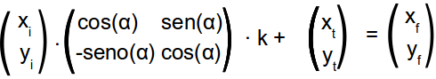
3.3.1.- EL DIBUJO EN PLANTA / DRAWING PLANT
El
trazado equivalente en planta es bastante sencillo ya que sólo se
necesita obviar el dato de la cota (excepto para el orden del dibujo
y de esa manera conoce que va arriba y abajo) y la transformación
requerida sólo es modificación de escala, giro y traslación:
The equivalent layout in plan is quite easy as only need to ignore the data dimension (except for the drawing order and thus knows that goes up and down) and the required transformation is only modification of scale, rotation and translation :
Pi
· G · k + T = Pf
G:
Aplica el giro del azimut real
k:
Pasará de metros a píxeles de pantalla.
T:
Colocará el punto de observación en el centro de la pantalla.
G: Apply the actual azimuth rotation
k: will pass from meters to screen pixels.
T: will place the observation point in the center of the screen.
3.3.2.- EL DIBUJO EN PERSPECTIVA / DRAWING IN PERSPECTIVE
Como ya se ha visto en 2.7, figura 3.3.2.a, el primer problema queda resuelto con la transformación de un punto 3D a uno 2D cónica (aérea) en el plano de comparación, Posteriormente una transformación de escala y otra de traslación lo colocarán correctamente en la pantalla.As already seen in 2.7, Figure 3.3.2.a, the first problem is solved with the transformation of a 3D point one 2D conic (aerial) in the plane of comparison, later a transformation of scale and other translational what be placed correctly on the screen.
 |
| Figura 3.3.2.a: Definición de los elementos que componen el dibujo en perspectiva cónica. Figure 3.3.2.a: Definition of the elements conical perspective drawing. |
Las
diversas fórmulas algebraicas siguen el siguiente proceso:
1º Se
conoce C, punto centro del proceso, a una distancia dPC en
la dirección de eje anterior se sitúa P. La cota superior óptima
está en torno a los 9 metros por encima de C (pero debe ser
modificable), por ello 9 metros será el valor por defecto.
2º A
una distancia determinada se localizará P. Es fácil, conociendo los
diversos puntos del eje, se conoce el vector de dirección y por ello
P=C+d·v/|v|. La distancia óptima está en torno a los 20 metros
(pero debe ser modificable)., por ello 20 metros será el valor por
defecto.
3º
Conocido el vector (Pxy,Cxy) se establece el plano de comparación
vertical:
(Px-Cx)
· y - (Py-Cy) · x + c = 0 ↔
a · x – b · y + c
= 0
4º Se
traza la recta de P-R: recta que pasa por dos puntos
5º Se
halla el punto de corte entre la recta P-R y se busca el punto de
corte, Q
6º Se
calculan las coordenadas relativas en al plano de comparación
(respecto al punto C, por ejemplo.
7º Se
realizan las transformaciones de semejanza necesarias para adaptarlo
a la pantalla.
Este
proceso se repite para todos los puntos de la explanada y se vuelve a
repetir para todos los puntos del terreno.
Anteriormente
se deciden cuales van a ser los pk y ejes visibles. Un punto óptimo
está el el rango de los 500 metros, para una altura del observados
de 9 metros. También debe ser modificable. La figura 3.3.2.b incluye
un esquema general del proceso de dibujo.
1 is known C, center point of the process, a dPC distance in the direction of the front axle stands P. The optimal upper bound is around 9 meters above C (but must be changed), so nine meters will be the default.
2 At a certain distance will be located P. It is easy, knowing the various points of the axis, the direction vector is known and therefore P=C+d·v/| v |. The optimal distance is around 20 meters (but must be changed)., So 20 meters is the default.
Known 3rd vector (Pxy, Cxy) vertical plane comparison is made:
(Px-Cx)·y-(Py-Cy)·x+c=0 ↔ a·x-b·y+c=0
Line through two points: 4th straight PR is drawn
5th the cutoff line is located between the PR and the cutoff is sought, Q
6 the relative coordinates are calculated in comparison to the plane (relative to the point C, for example.
7th similarity transformations necessary to fit the screen are performed.
This process is repeated for all points of the Esplanade and is repeated for all points of the terrain.
Previously decide which will be the pk and visible axes. An optimum is the range of 500 meters to a height of 9 meters observed. It should also be modified. 3.3.2.b The figure includes an overview of the drawing process.
 |
Figura
3.3.2.b:
Diagrama de la estructura general del proceso de dibujo
Figure 3.3.2.b: Diagram of the general structure of the process of drawing
|
Al
final, como se observa en la figura 3.3.2.c, se muestra un ejemplo
del resultado del proceso de dibujo.
At the end, as seen in Figure 3.3.2.c, an example of a result of the drawing is shown.
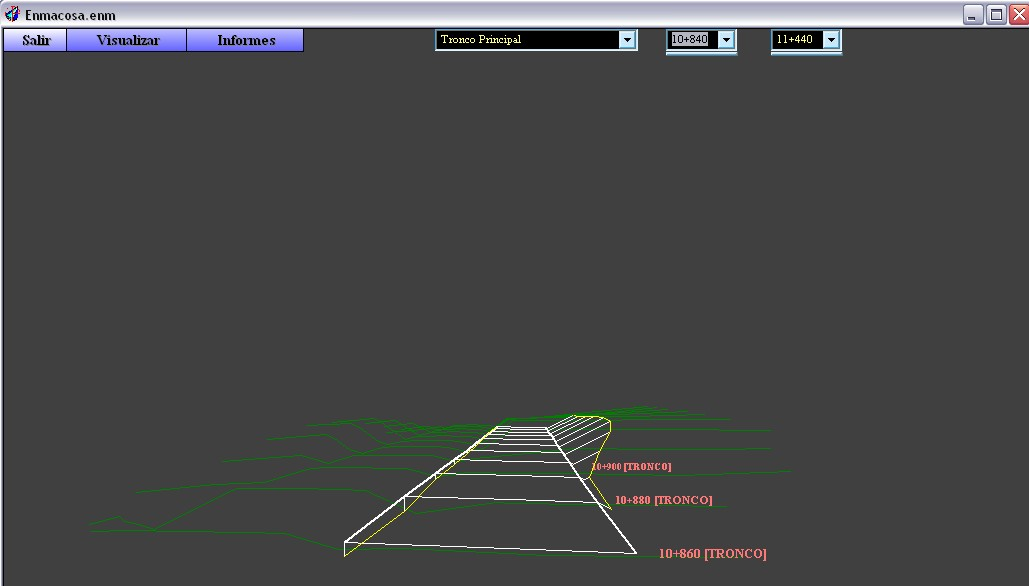 |
| Figura 3.3.2.c: Resultado del dibujo Figure 3.3.2.c: Result drawing |
La
elección del Eje y del Pk sitúa el punto de observación.
+
Los puntos situados detrás del observador también originan una
recta de corte por lo que se puede originar un “efecto espejo”
que debe ser evitado. La forma de hacerlo es la siguiente, el plano
de comparación, de ecuación ax+by+c=0 se convierte en la función
f=ax+by+c, si se sustituye (x,y) por los valores del punto P ésta
nos dará un valor positivo o negativo. Sólo se tienen que dibujar
aquellos puntos que den en esta función distinto signo al anterior.
+
Aunque a continuación se materializan los resultados en código de
Visual Basic puede ser transcrito en cualquier otro lenguaje con sus
respectivas correcciones sintácticas. Lo importante es la resolución
pormenorizada de todas y cada una de las ecuaciones algebraicas
propuestas con anterioridad.
Choosing Pk Axis and placed the observation point.
+ The points behind the observer also originate a straight cut so can cause a "mirror effect" should be avoided. The way is the following, the comparison plane, equation ax + by + c = 0 becomes f = ax + by + c function, if substituted (x, y) by the values of point P it will give a positive or negative value. You only need to draw the points that give this function than the previous sign.
+ Even then the results are embodied in Visual Basic code can be transcribed in any other language with their syntactic corrections. What matters is the depth resolution of each and every one of algebraic equations proposed previously.
Para
entender el proceso seguido se explica la programación en la
siguiente secuencia:
Para la lectura inicial de datos:
→ Subrutina Abrir → Subrutinas Lee_Bases_Datos, y Lee_Ejes
Para la visualización de estos:
→ Subrutina Recorrido → Subrutinas Lee_Bases_Datos, Lee_Ejes y Lee_Estructuras
Para ambos casos:
→ Subrutina Lee_Ejes → Leo_Uno_A_Uno
→ Subrutina Leo_Uno_A_Uno → Saltaor
- _____________________
(NOTA: Los siguiente códigos están en VB o C)
Private
Sub Abrir()
'Se
busca el directorio que contiene datos
cmd.DialogTitle
= "Importar"
cmd.FileName
= "": cmd.CancelError = True
cmd.Filter
= "Proyectos (*.enm)|*.enm|Todos los ficheros|*.*"
cmd.FilterIndex
= 1: cmd.Action = 1: Directorio = cmd.InitDir: Directorio =
cmd.FileName
'Se
abre el directorio que contiene datos
Do
Directorio
= Left(Directorio, Len(Directorio) - 1)
Loop
Until Right(Directorio, 1) = "\"
Grupo_Ejes.Path
= Directorio: Grupo_Ejes.Pattern = "*.ter"
'Se
leen las bases de datos desde la sub-rutina Lee_Bases_Datos
Lee_Bases_Datos
'Se
lee el trazado desde la sub-rutina Lee_Ejes
Lee_Ejes
'Se
leen las estructuras del entorno, la sub-rutina Lee_Estructuras
Lee_Estructuras
'Se
leen los detalles desde la sub-rutina Lee_Detalles
Lee_Detalles
'Se
elije el modo de visualización inicial
VisualizarEn3D
End
Sub
_____________________
Private
Sub Lee_Bases_Datos()
'Se
inicializa Densidades
Data1.Connect
= DBI_Connect
Data1.DatabaseName
= DBI_Densidad
'Data1.RecordSource
= "SELECT * FROM densidad ORDER BY PK"
'Data1.Refresh
'Se
inicializa Suelos
Data2.DatabaseName
= DBI_Suelos
Data2.RecordSource
= "SELECT * FROM [" & DBT_Suelos & "] ORDER BY
PK"
Data2.Refresh
'Se
inicializan las fotos
Data3.Connect
= DBI_Connect
Data3.DatabaseName
= DBI_Fotos
Data3.RecordSource
= DBT_Fotos
'Se
inicializan los firmes
..
estructuras
..
fotos
..
End
Sub
_____________________
Private
Sub Lee_Ejes()
'Se
lee el grupo de ejes
For
H = 1 To Grupo_Ejes.ListCount
Archivo = Elemento(H)
Plataforma = Archivo +
".plataforma"
Eje = Archivo + ".eje"
Terreno = Archivo + ".ter"
N = Leo_Uno_A_Uno(Archivo,
Terreno, Plataforma, Eje, H)
Next
Himno
End
Sub
_____________________
Sub
Lee_Estructuras()
Data4.RecordSource
= "SELECT DISTINCT ESTRUCTRUR FROM BD_Estructuras WHERE {
distancia( Xv, CENTROX, Yv, CENTROY)< entorno }
'
Esta es el punto más importante Xv, Yv Son las coordenadas del punto
de vista y entorno, el máximo campo visible
Data4.Refresh
: Data4.Recordset.MoveFirst
Do
Load
Nombre_Estructura(Data4.Recordset(0) )
'
Previamente se definió Nombre_Estructura como una matriz de objetos
botón
Data4.Recordset.MoveNext
Loop
Until Data4.Recordset.EOF
End
Sub
_____________________
Private
Function Leo_Uno_A_Uno(ByVal nom As String, ByVal ter As String,
ByVal pla As String, ByVal eje As String, ByVal N As Integer) As
Integer
NombreEje(N)
= nom
Dim
LineaT, LineaP, LineaC As String
'==========================================
'
LO PRIMERO SERÁ CALCULAR EL NÚMERO DE PKS
'==========================================
Open
Directorio + pla For Input As #2
50:
Line Input #2, LineaP: If EOF(2) Then GoTo 60
If
LineaP Like "*PS*" Then Line
Input #2, LineaP: GoTo 50
If
LineaP Like "*[0-9].[0-9][0-9]*"
Then
If
Left(LineaP, 7) = " ispol" Then ChivatoIstram = 1: z =
Zinicio2(nom, ter, pla, eje, N): Exit Function
If
ChivatoIstram <> 1 Then
ClipIIIAntiguo
= InStr(LineaP, Tablu)
If
ClipIIIAntiguo = 0 Then 'diferenciacion entre el clip normal o el de
windows
Vol
= Val(Left(LineaP, 18))
If
Vol = 0 And I <> 0 Then GoTo 50
If
Vol <= Vol1 Then GoTo 50
If
Vol <> Int(Vol) Then GoTo 50
Vol1
= Vol
indice_pk(N,
I) = Vol
Dist_p(N,
0, I) = Val(Mid(LineaP, 27, 10))
Dist_p(N,
1, I) = Val(Mid(LineaP, 37, 10))
Dist_p(N,
2, I) = Val(Mid(LineaP, 47, 10))
Dist_p(N,
3, I) = Val(Mid(LineaP, 67, 10))
Dist_p(N,
4, I) = Val(Mid(LineaP, 77, 10))
Dist_p(N,
5, I) = Val(Mid(LineaP, 97, 10))
Dist_p(N,
6, I) = Val(Mid(LineaP, 107, 10))
Dist_p(N,
7, I) = Val(Mid(LineaP, 117, 10))
Cota_p(N,
0, I) = Val(Mid(LineaP, 27, 10))
Cota_p(N,
1, I) = Val(Mid(LineaP, 37, 10))
Cota_p(N,
2, I) = Val(Mid(LineaP, 47, 10))
Cota_p(N,
3, I) = Val(Mid(LineaP, 67, 10))
Cota_p(N,
4, I) = Val(Mid(LineaP, 77, 10))
Cota_p(N,
5, I) = Val(Mid(LineaP, 97, 10))
Cota_p(N,
6, I) = Val(Mid(LineaP, 107, 10))
Cota_p(N,
7, I) = Val(Mid(LineaP, 117, 10))
Else
indice_pk(N,
I) = Vol
Primeo
= InStr(Primeo + 1, LineaP, Tablu, vbBinaryCompare): If Primeo + 1 =
InStr(Primeo + 1, LineaP, Tablu, vbBinaryCompare) Then Primeo =
InStr(Primeo + 1, LineaP, Tablu, vbBinaryCompare)
Dist_p(N,
0, I) = Val(Mid(LineaP, Primeo, 7))
Primeo
= InStr(Primeo + 1, LineaP, Tablu, vbBinaryCompare): If Primeo + 1 =
InStr(Primeo + 1, LineaP, Tablu, vbBinaryCompare) Then Primeo =
InStr(Primeo + 1, LineaP, Tablu, vbBinaryCompare)
Dist_p(N,
1, I) = Val(Mid(LineaP, Primeo, 7))
Primeo
= InStr(Primeo + 1, LineaP, Tablu, vbBinaryCompare): If Primeo + 1 =
InStr(Primeo + 1, LineaP, Tablu, vbBinaryCompare) Then Primeo =
InStr(Primeo + 1, LineaP, Tablu, vbBinaryCompare)
Dist_p(N,
2, I) = Val(Mid(LineaP, Primeo, 7))
Primeo
= InStr(Primeo + 1, LineaP, Tablu, vbBinaryCompare): If Primeo + 1 =
InStr(Primeo + 1, LineaP, Tablu, vbBinaryCompare) Then Primeo =
InStr(Primeo + 1, LineaP, Tablu, vbBinaryCompare)
Dist_p(N,
3, I) = Val(Mid(LineaP, Primeo, 7))
Primeo
= InStr(Primeo + 1, LineaP, Tablu, vbBinaryCompare): If Primeo + 1 =
InStr(Primeo + 1, LineaP, Tablu, vbBinaryCompare) Then Primeo =
InStr(Primeo + 1, LineaP, Tablu, vbBinaryCompare)
Dist_p(N,
4, I) = Val(Mid(LineaP, Primeo, 7))
Primeo
= InStr(Primeo + 1, LineaP, Tablu, vbBinaryCompare): If Primeo + 1 =
InStr(Primeo + 1, LineaP, Tablu, vbBinaryCompare) Then Primeo =
InStr(Primeo + 1, LineaP, Tablu, vbBinaryCompare)
Dist_p(N,
5, I) = Val(Mid(LineaP, Primeo, 7))
Primeo
= InStr(Primeo + 1, LineaP, Tablu, vbBinaryCompare): If Primeo + 1 =
InStr(Primeo + 1, LineaP, Tablu, vbBinaryCompare) Then Primeo =
InStr(Primeo + 1, LineaP, Tablu, vbBinaryCompare)
Dist_p(N,
6, I) = Val(Mid(LineaP, Primeo, 7))
Primeo
= InStr(Primeo + 1, LineaP, Tablu, vbBinaryCompare): If Primeo + 1 =
InStr(Primeo + 1, LineaP, Tablu, vbBinaryCompare) Then Primeo =
InStr(Primeo + 1, LineaP, Tablu, vbBinaryCompare)
Dist_p(N,
7, I) = Val(Mid(LineaP, Primeo, 7))
If
Abs(Dist_p(N, 3, I) - Dist_p(N, 2, I)) > 20 Then Dist_p(N, 3, I) =
0
If
Abs(Dist_p(N, 4, I) - Dist_p(N, 5, I)) > 20 Then Dist_p(N, 4, I) =
0
Cota_p(N,
0, I) = Val(Mid(LineaP, Primeo, 8))
Primeo
= InStr(Primeo + 1, LineaP, Tablu, vbBinaryCompare): If Primeo + 1 =
InStr(Primeo + 1, LineaP, Tablu, vbBinaryCompare) Then Primeo =
InStr(Primeo + 1, LineaP, Tablu, vbBinaryCompare)
Cota_p(N,
1, I) = Val(Mid(LineaP, Primeo, 8))
Primeo
= InStr(Primeo + 1, LineaP, Tablu, vbBinaryCompare): If Primeo + 1 =
InStr(Primeo + 1, LineaP, Tablu, vbBinaryCompare) Then Primeo =
InStr(Primeo + 1, LineaP, Tablu, vbBinaryCompare)
Cota_p(N,
2, I) = Val(Mid(LineaP, Primeo, 8))
Primeo
= InStr(Primeo + 1, LineaP, Tablu, vbBinaryCompare): If Primeo + 1 =
InStr(Primeo + 1, LineaP, Tablu, vbBinaryCompare) Then Primeo =
InStr(Primeo + 1, LineaP, Tablu, vbBinaryCompare)
Cota_p(N,
3, I) = Val(Mid(LineaP, Primeo, 8))
Primeo
= InStr(Primeo + 1, LineaP, Tablu, vbBinaryCompare): If Primeo + 1 =
InStr(Primeo + 1, LineaP, Tablu, vbBinaryCompare) Then Primeo =
InStr(Primeo + 1, LineaP, Tablu, vbBinaryCompare)
Cota_p(N,
4, I) = Val(Mid(LineaP, Primeo, 8))
Primeo
= InStr(Primeo + 1, LineaP, Tablu, vbBinaryCompare): If Primeo + 1 =
InStr(Primeo + 1, LineaP, Tablu, vbBinaryCompare) Then Primeo =
InStr(Primeo + 1, LineaP, Tablu, vbBinaryCompare)
Cota_p(N,
5, I) = Val(Mid(LineaP, Primeo, 8))
Primeo
= InStr(Primeo + 1, LineaP, Tablu, vbBinaryCompare): If Primeo + 1 =
InStr(Primeo + 1, LineaP, Tablu, vbBinaryCompare) Then Primeo =
InStr(Primeo + 1, LineaP, Tablu, vbBinaryCompare)
Cota_p(N,
6, I) = Val(Mid(LineaP, Primeo, 8))
Primeo
= InStr(Primeo + 1, LineaP, Tablu, vbBinaryCompare): If Primeo + 1 =
InStr(Primeo + 1, LineaP, Tablu, vbBinaryCompare) Then Primeo =
InStr(Primeo + 1, LineaP, Tablu, vbBinaryCompare)
Cota_p(N,
7, I) = Val(Mid(LineaP, Primeo, 8))
If
Abs(Cota_p(N, 3, I) - Cota_p(N, 2, I)) > 1 Then Cota_p(N, 3, I) =
Cota_p(N, 2, I)
If
Abs(Cota_p(N, 4, I) - Cota_p(N, 5, I)) > 1 Then Cota_p(N, 4, I) =
Cota_p(N, 5, I)
Else
indice_pk(N,
I) = Vol
Dist_p(N,
0, I) = Cuanto_es(Mid(LineaP, 41, 9))
Dist_p(N,
1, I) = Cuanto_es(Mid(LineaP, 41, 9))
Dist_p(N,
2, I) = Cuanto_es(Mid(LineaP, 14, 9))
Dist_p(N,
3, I) = Cuanto_es(Mid(LineaP, 14, 9))
Dist_p(N,
4, I) = Cuanto_es(Mid(LineaP, 14, 9))
Dist_p(N,
5, I) = Cuanto_es(Mid(LineaP, 60, 9))
Dist_p(N,
6, I) = Cuanto_es(Mid(LineaP, 60, 9))
Dist_p(N,
7, I) = Cuanto_es(Mid(LineaP, 60, 9))
Dist_p(N,
8, I) = Cuanto_es(Mid(LineaP, 87, 9))
Dist_p(N,
9, I) = Cuanto_es(Mid(LineaP, 87, 9))
Cota_p(N,
0, I) = Cuanto_es(Mid(LineaP, 50, 9))
Cota_p(N,
1, I) = Cuanto_es(Mid(LineaP, 50, 9))
Cota_p(N,
2, I) = Cuanto_es(Mid(LineaP, 23, 9))
Cota_p(N,
3, I) = Cuanto_es(Mid(LineaP, 23, 9))
Cota_p(N,
4, I) = Cuanto_es(Mid(LineaP, 23, 9))
Cota_p(N,
5, I) = Cuanto_es(Mid(LineaP, 69, 9))
Cota_p(N,
6, I) = Cuanto_es(Mid(LineaP, 69, 9))
Cota_p(N,
7, I) = Cuanto_es(Mid(LineaP, 69, 9))
Cota_p(N,
8, I) = Cuanto_es(Mid(LineaP, 96, 9))
Cota_p(N,
9, I) = Cuanto_es(Mid(LineaP, 96, 9))
End
If
End
If
GoTo
50
60:
Close #2
indice_pk(N,
I) = -1 'ESTA PAUTA SEÑALA EL FINAL DE LOS DATOS
I
= I - 1
'==========================================
'
LO SEGUNDO RELLENAR LAS VARIBLES CON I PKS
'==========================================
Open
Directorio + ter For Input As #1
'
LEEREMOS EL TERRENO
V
= indice_pk(N, 0) - 1
Line
Input #1, LineaT ' PARA DESHACERNOS DE LA LECTURA DE "*TER"
For
j = 0 To I
If
V < indice_pk(N, j) Then Line Input #1, LineaT: If EOF(1) Then
GoTo 62
V
= Val(LineaT)
If
V = indice_pk(N, j) Then
VFinal
= Val(Right(LineaT, Len(LineaT) - InStr(1, LineaT, ",",
0)))
Line
Input #1, LineaT: If EOF(1) Then GoTo 62
Dedo
= InStr(1, LineaT, ",", 0)
Cota_t(N,
1, j) = Val(Right(LineaT, Len(LineaT) - Dedo))
Dist_t(N,
1, j) = Val(LineaT)
VInicial
= 2
For
k = VInicial To VFinal
Line
Input #1, LineaT: If EOF(1) Then GoTo 62
Dedo
= InStr(1, LineaT, ",", 0)
'
Print si; la; Cota; inferior; es; tal; cual
Cota_t(N,
k, j) = Val(Right(LineaT, Len(LineaT) - Dedo))
Dist_t(N,
k, j) = Val(LineaT)
Next
k
If
Dist_t(N, VFinal, j) < Dist_p(N, 7, j) Then
Dist_t(N,
VFinal + 1, j) = Dist_p(N, 7, j) + 10
Cota_t(N,
VFinal + 1, j) = Cota_t(N, VFinal, j)
VInicial
= 3 ' Stop
End
If
End
If
Next
j
'----------------------
'
TERMINEMOS CON EL EJE
'----------------------
Open
Directorio + eje For Input As #3
For
j = 0 To I
Do
Line
Input #3, LineaC
If
Len(LineaC) < 7 Then GoTo 63
If
LineaC Like "*P*" Then GoTo 63
If
LineaC Like "*===*" Then GoTo 63
Loop
Until InStr(1, LineaC, Trim(indice_pk(N, j)), 0) <> 0
If
ClipIIIAntiguo = 0 Then
Y_eje(N,
j) = Cuanto_es(Mid(LineaC, 33, 11))
If
Y_eje(N, j) = 0 Then GoTo 63
X_eje(N,
j) = Cuanto_es(Mid(LineaC, 21, 10))
If
MinimaX > X_eje(N, j) Then MinimaX = X_eje(N, j)
If
MinimaY > Y_eje(N, j) Then MinimaY = Y_eje(N, j)
If
MaximaX < X_eje(N, j) Then MaximaX = X_eje(N, j)
If
MaximaX < Y_eje(N, j) Then MaximaY = Y_eje(N, j)
Beta(N,
j) = Cuanto_es(Mid(LineaC, 47, 8))
Betty
= Betty + Beta(N, j) / 100
Else
Y_eje(N,
j) = Cuanto_es(Mid(LineaC, 18, 11))
If
Y_eje(N, j) = 0 Then GoTo 63
X_eje(N,
j) = Cuanto_es(Mid(LineaC, 7, 10))
If
MinimaX > X_eje(N, j) Then MinimaX = X_eje(N, j)
If
MinimaY > Y_eje(N, j) Then MinimaY = Y_eje(N, j)
If
MaximaX < X_eje(N, j) Then MaximaX = X_eje(N, j)
If
MaximaX < Y_eje(N, j) Then MaximaY = Y_eje(N, j)
Beta(N,
j) = Val(Mid(LineaC, 30, 8))
Betty
= Betty + Beta(N, j) / 100
End
If
Next
j
Close
#3
Zinicio
= I
End
Function
_____________________
Sub
Recorrido
'Combo1
Lista desplegable con los nombres del eje
'Combo2
Lista desplegable con los pks del recorrido del eje anterior
Indice
= Combo2.ListIndex
ColDat
= Combo1.ListIndex
'================================================================
'
======== DEFINICION DEL PLANO DE COMPARACION =======
'================================================================
Cota_Ini = Cota_p(ColDat, 3,
Indice) 'Pone a la altura de 6000 el eje central
Xe = X_eje(ColDat, Indice)
Ye = Y_eje(ColDat, Indice)
Ze = Cota_Ini
Alfa
= Giro / 200 * 3.14159265358979 + (-Beta(ColDat, Indice)) / 100 *
1.5707963267949
'================================================================
'
======== DEFINICION DEL PUNTO DE VISTA =======
'================================================================
Xv = Xe + Dis * Sin(Alfa)
Yv = Ye - Dis * Cos(Alfa)
Zv = Altura
mm = Tan(-1.5707963267949 +
Alfa)
nn = Yv - Xv * mm
M = Tan(Alfa)
N = Ye - Xe * M
'================================================================
'
======== EMPEZANDO A SALTAR ========
'================================================================
For I = Indice To Indice +
Saltos * Signal Step Signal
Y = Saltaor(Indice,
ColDat, I)
Next I
barra = Val(Combo2) * 1000 +
Val(Right(Combo2, 3))
For j = 1 To Saltos
Radio
= (10 * Saltos): Pej = 0
For I = 0 To Dimensiones
For k = 0 To Numeral
Equis = X_eje(I, k):
If Equis = 0 Then k = Numeral
If Abs(Equis - Xv) + Abs(Y_eje(I, k) - Yv) < Radio Then
Y =
Saltaor(Indice, I, k)
'
Esta referencia a la función Saltaor es para acceder rápidamente a
los datos del entorno al pk)
End If
Next k
End
If
End
Sub
_____________________
Function
Saltaor(ByVal pekfin As Integer, ByVal ColDat As Integer, ByVal I As
Integer) As Integer
'***********************************************
'
********* TERRENO ********
'***********************************************
For j = 0 To 20
D = Dist_t(ColDat, j, I)
Bet = 0 * Giro / 200 *
3.14159265358979 + (-Beta(ColDat, I)) / 100 * 1.5707963267949
Oa = D * Cos(Bet) +
X_eje(ColDat, I)
Ob = D * Sin(Bet) +
Y_eje(ColDat, I)
Oc = Cota_t(ColDat, j, I)
If Oc <> 0 Then
Chato = PuntOstias(Oa,
Ob, Oc)
If Chato = 1 Then
If j = 0 Then
Uu = Coor_X:
Vv = Coor_Y
Else
Colore =
QBColor(2)
Xx = Coor_X:
Yy = Coor_Y
l = recta(Uu,
Vv, Xx, Yy, Colore)
Uu = Xx: Vv =
Yy
End If
End If
End If
Next j
'***********************************************
' *********
PLATAFORMA ********
'***********************************************
For j = 0 To 9
D = Dist_p(ColDat, j, I): If
D > 100 Then Exit For
Bet = 0 * Giro / 200 *
3.14159265358979 + (-Beta(ColDat, I)) / 100 * 1.5707963267949
Oa = D * Cos(Bet) +
X_eje(ColDat, I)
Ob = D * Sin(Bet) +
Y_eje(ColDat, I)
Oc = Cota_p(ColDat, j, I)
If Oc <> 0 Then
Chato = PuntOstias(Oa, Ob,
Oc)
If Chato = 1 Then
If j = 0 Then
Uu = Coor_X: Vv = Coor_Y
mimi(0, I - Iluso) = Uu:
nini(0, I - Iluso) = Vv
Else
Colore = QBColor(15)
Xx = Coor_X: Yy = Coor_Y
If j = 2 Then mimi(1, I -
Iluso) = Xx: nini(1, I - Iluso) = Yy
l = recta(Uu, Vv, Xx,
Yy, Colore)
If j = 5 Then mimi(2, I
- Iluso) = Xx: nini(2, I - Iluso) = Yy
If j = 7 Then
mimi(3, I - Iluso) =
Xx: nini(3, I - Iluso) = Yy
Dedo = Dcia(Oa, Ob,
Xv, Yv)
If
Planta.Caption = "Ver Planta" Then
If Dedo < 100
Then
Picture1.CurrentX =
Xx + 50
Picture1.CurrentY =
Yy - 250
Picture1.ForeColor
= RGB(255, 120, 120)
Picture1.FontSize =
Int(70 / Sqr(Dedo))
Picture1.FontName =
"times"
Picture1.Print
Format(indice_pk(ColDat, I), "0+000");
Picture1.Print
Texto
End If
Else
Funx = (Xx + 50) /
Escala_Pitufo
Funy = (Yy - 250) /
Escala_Pitufo
Picture1.ForeColor
= RGB(255, 120, 120)
If ColDat =
Combo1.ListIndex Then
Picture1.ForeColor
= QBColor(14): Gordito = 125 / Saltos
If I =
Combo2.ListIndex Then Picture1.ForeColor = QBColor(15): Gordito = 200
/ Saltos
Else
End If
End
If
End If
Uu = Xx: Vv = Yy
End If
End If
End If
Next j
End
Function
3.3.2.1.- EL DIBUJO CON SUPERFICIES PLANAS / DRAWING WITH FLAT SURFACES
El dibujo en 3D con líneas es más sencillo que el propio dibujo en 3D con superficies planas (renderizado) la dificultad añadida está en agrupar los puntos de tres en tres (triangulación) a los puntos más cercanos por concepto o una simple triangulación de Delaunay. El problema está en el tiempo de cálculo añadido que se necesita en esta serie de operaciones.
La disminución del tiempo se obtiene de dos maneras, Cambiando el lenguaje y la forma de operar
Todos los lenguajes de alto nivel permiten llamadas a comandos, o, incluso a otros programas externos que actuarán como subrutinas de este. Desde VB se hace a través de la función Shell() y en PHP desde las funciones exec(), system() y alguna más.
Para que esta parte sea lo más rápida posible se realizará en C y el ejecutable se creará con el programa gratuito gcc disponible para Linux y Windows. De esta manera se tendrá un mismo programa que podrá ser compilado para cualquier sistema operativo.
De todas maneras los bucles con demasiado numerosos,: el 1º, 2º y 3º recorre los puntos hasta localizar los puntos más cercanos, el 4º, 5º y 6º compara estos puntos con los anteriores para saber su posición respecto a los anteriores ya calculados para saber si están delante o detrás del resto, total o parcialmente, y un 7º para conocer según su orientación el color iluminado.
Estas operaciones comparativas de posición pueden provocar reiterados anidamientos y éstos lentitud en la respuesta hacia el dibujo final.
Las primeras versiones hicieron el trabajo excesivamente lento hasta que se incluyeron en la programación las “sintegrales”.(Véase apartado 3.6.3) .
Si se analiza alguno de los bucles y dentro de él las operaciones que se realizan son lo suficientemente rutinarias puede extrapolarse el término general y sustituirse éste por el bucle. No se eliminarán todos pero sí una gran parte:
Uniendo ambos criterios se crea el siguiente programa en C (se realiza en C para añadir velocidad en la ejecución del programa una vez compilado):
The 3D drawing lines is simpler than the drawing itself in 3D with flat surfaces (rendering) the added difficulty is to combine the points in threes (triangulation) to the closest for concept or a simple Delaunay triangulation points. The problem is added computation time is needed in this series of operations.
The decrease in time is obtained in two ways, changing the language and how to operate
All high-level languages allow calls to commands, or even to other external programs to act as subroutines of this. From VB is done through the Shell () function in PHP from the exec (), system () and some more.
For this part as fast as possible will be made in C and the executable is created with the free gcc available for Linux and Windows. Thus the same program can be compiled for any operating system will have.
Anyway loops with too many,: the 1st, 2nd and 3rd runs through the points to locate the nearest points, 4th, 5th and 6th compares these points with the above to find your position on the above and calculated to know if they are in front or behind other, wholly or partially, and a 7th to know by color illuminated orientation.
These comparative operations can cause repeated nesting position and these slow response to the final drawing.
Early versions made excessively slow work until the schedule included in the "sintegrales." (See section 3.6.3).
If we analyze some of the loops and within it the operations performed are sufficiently routine can be extrapolated the general term and replaced it by the loop. Not all but eliminated much:
Uniting both criteria the following program is created in C (done in C to add speed program execution once compiled):
 |
| Figura 3.3.2.1.a: Resultado del dibujo con triángulos sólidos. Figure 3.3.2.1.a: Result of the drawing with solid triangles. |
3.3.2.2.- EL DIBUJO EN EL NAVEGADOR / DRAWING IN THE BROWSER
La posibilidad de realizar el dibujo gráfico en el navegador sigue siendo demasiado lenta pero para exponer la forma de hacerlo sería a través de javascript con la definición de elementos DIV a sólo píxeles. El hecho de crear todo un objeto del DOM de HTML para dibujar un punto y que este deba ser controlado a través de javascript (lenguaje intérprete) dentro del navegador, y éste, dentro del S.O. Hace que éste sistema se vuelva demasiado lento. La siguiente visualización (figura 3.3.2.2) tarda unos 3 minutos en renderizarse:
The possibility of graph drawing in the browser is still too slow but to expose the way would be through javascript with the definition of DIV elements just pixels. The fact create an entire HTML DOM object to draw a point and that this should be controlled through javascript (language interpreter) within the browser, and this, in the SO Makes this system becomes too slow. The following display (Figure 3.3.2.2) takes about 3 minutes rendered:
 |
| Figura 3.3.2.2: Resultado del dibujo con Javascript Figure 3.3.2.2: Result of the drawing with Javascript |
El
código para la obtención del dibujo anterior (figura 3.3.2.2) sería
al siguiente. Se ha substituido los elementos redundantes por puntos
suspensivos.
(NOTA: HTML y PHP)
<!DOCTYPE
HTML PUBLIC
"-//W3C//DTD HTML 4.0 Transitional//EN">
<!--
saved from url=(0046)file://\\oc-proyecto\interno\www\idi\3d\3d.htm
-->
<!--
saved from url=(0045)http://www.lutanho.net/svgvml3d/platonic.html
--><HTML
xmlns:v
= "urn:schemas-microsoft-com:vml"><HEAD><TITLE>SVG-VML-3D-Example
- Platonic Solids</TITLE>
<META
http-equiv=Content-Type
content="text/html;
charset=windows-1252">
<STYLE>v\:*
{BEHAVIOR: url(#default#VML)}
INPUT
{FONT-SIZE: 14pt; WIDTH: 28px; FONT-FAMILY: 'Times New Roman';
HEIGHT: 28px; BACKGROUND-COLOR:#c0c0ff}
</STYLE>
<SCRIPT
language=JavaScript
src="SVG-VML-3D-Example%20-%20Platonic%20Solids_archivos/svgvml3d.js"
type=text/javascript></SCRIPT>
<SCRIPT
language=JavaScript
src="SVG-VML-3D-Example%20-%20Platonic
%20Solids_archivos/platonic.js" type=text/javascript></SCRIPT>
<SCRIPT
language=JavaScript
type=text/javascript>
var
S,
T, O, C, I, D;
function
Init()
{ if
(useSVG){
if
(!
SVGObjects[0]){
setTimeout("Init()",100);
return;
} S=new
Scene3D(SVGObjects[0],0,500,500);
}
else
S=new
Scene3D(document.getElementById("Scene1"),1);
T
= new
Trian(S,"#A20000","
#00ff00","",1,0,0,0,0,0,0,0,0,0);
T
= new
Trian(S,"#008400","
#00ff00","",1,-1.21638424538891,-1.87847702892497,3.438995E-02,-1.37859868711326,-1.97480649444275,2.437012ET
=
new
Trian(S,"#008300","
#00ff00","",1,-1.25176361426362,-1.81815704993904,3.33200073242187E-02,-1.37859868711326,-1.97480649444275,2.
…
C
= new
Plano
(S,"#85EEEE","#85EEEE","",1,-1.57154412898468,-1.27294794804417,0.022919921875,-1.61606559153064,-1.197041176
C
= new
Plano
(S,"#77CACA","#77CACA","",1,-1.61606559153064,-1.19704117608257,-5.25299072265625E-02,-1.64333499144181,-1.15
…
}
</SCRIPT>
<META
content="MSHTML
6.00.5730.13" name=GENERATOR></HEAD>
<BODY
bgColor=#0000ff><INPUT
title="zoom
picture in" onclick=ZoomPicture(1)
type=button
value=[+]>
<SCRIPT
language=JavaScript>
if
(useSVG)
document.writeln("<embed
width='1000' height='800' name='Scene1' src='scene.svg'
wmode='transparent'
type='image/svg+xml' />");
else
document.writeln("<div
id='Scene1'
style='position:
relative;
width:1000;
height:800;
overflow:
hidden;'></div>");
</SCRIPT>
</TABLE></BODY></HTML>
**** TRATAMIENTO DE LA INFORMACIÓN / INFORMATION PROCESSING ****
3.4.- LA UNIÓN DEL TRAZADO CON LAS BASES DE DATOS / THE UNION OF ROUTE AND DATABASES
El trazado se une a las bases de datos de forma inmediata ya que todas las bases de datos (u hojas de cálculo) contienen dos campos uno dedicado al eje y el otro al pk. Las dos posibilidades de consulta son: BD → trazado, o , Trazado → BD.
En el primer caso, BD → trazado, sería una selección tipo de punto 3.3
En el segundo caso, Trazado → BD, se necesitaría una consulta del tipo:
SELECT * FROM BaseDeDatos WHERE PK=[pk buscado, o entorno] AND EJE=[eje buscado o entorno]
y la consulta habría sido realizada,.
The route joins the database immediately because all databases (or spreadsheet) contain two fields one dedicated to the axis and the other to pk. The two possibilities for consultation are: BD → route, or route → BD.
In the first case, BD → path, it would be a kind selection of point 3.3
In the second case, Route → BD, a query would need to type:
SELECT * FROM DATABASE WHERE PK = [pk sought, or environment] AND SHAFT = [axis sought or environment]
and consultation have been made,.
Continuará ...
To be continued ...
No hay comentarios:
Publicar un comentario